
11.6: Vapor Pressures of Volatile Binary Solutions
- Page ID
- 426479
\( \newcommand{\vecs}[1]{\overset { \scriptstyle \rightharpoonup} {\mathbf{#1}} } \)
\( \newcommand{\vecd}[1]{\overset{-\!-\!\rightharpoonup}{\vphantom{a}\smash {#1}}} \)
\( \newcommand{\id}{\mathrm{id}}\) \( \newcommand{\Span}{\mathrm{span}}\)
( \newcommand{\kernel}{\mathrm{null}\,}\) \( \newcommand{\range}{\mathrm{range}\,}\)
\( \newcommand{\RealPart}{\mathrm{Re}}\) \( \newcommand{\ImaginaryPart}{\mathrm{Im}}\)
\( \newcommand{\Argument}{\mathrm{Arg}}\) \( \newcommand{\norm}[1]{\| #1 \|}\)
\( \newcommand{\inner}[2]{\langle #1, #2 \rangle}\)
\( \newcommand{\Span}{\mathrm{span}}\)
\( \newcommand{\id}{\mathrm{id}}\)
\( \newcommand{\Span}{\mathrm{span}}\)
\( \newcommand{\kernel}{\mathrm{null}\,}\)
\( \newcommand{\range}{\mathrm{range}\,}\)
\( \newcommand{\RealPart}{\mathrm{Re}}\)
\( \newcommand{\ImaginaryPart}{\mathrm{Im}}\)
\( \newcommand{\Argument}{\mathrm{Arg}}\)
\( \newcommand{\norm}[1]{\| #1 \|}\)
\( \newcommand{\inner}[2]{\langle #1, #2 \rangle}\)
\( \newcommand{\Span}{\mathrm{span}}\) \( \newcommand{\AA}{\unicode[.8,0]{x212B}}\)
\( \newcommand{\vectorA}[1]{\vec{#1}} % arrow\)
\( \newcommand{\vectorAt}[1]{\vec{\text{#1}}} % arrow\)
\( \newcommand{\vectorB}[1]{\overset { \scriptstyle \rightharpoonup} {\mathbf{#1}} } \)
\( \newcommand{\vectorC}[1]{\textbf{#1}} \)
\( \newcommand{\vectorD}[1]{\overrightarrow{#1}} \)
\( \newcommand{\vectorDt}[1]{\overrightarrow{\text{#1}}} \)
\( \newcommand{\vectE}[1]{\overset{-\!-\!\rightharpoonup}{\vphantom{a}\smash{\mathbf {#1}}}} \)
\( \newcommand{\vecs}[1]{\overset { \scriptstyle \rightharpoonup} {\mathbf{#1}} } \)
\( \newcommand{\vecd}[1]{\overset{-\!-\!\rightharpoonup}{\vphantom{a}\smash {#1}}} \)
\(\newcommand{\avec}{\mathbf a}\) \(\newcommand{\bvec}{\mathbf b}\) \(\newcommand{\cvec}{\mathbf c}\) \(\newcommand{\dvec}{\mathbf d}\) \(\newcommand{\dtil}{\widetilde{\mathbf d}}\) \(\newcommand{\evec}{\mathbf e}\) \(\newcommand{\fvec}{\mathbf f}\) \(\newcommand{\nvec}{\mathbf n}\) \(\newcommand{\pvec}{\mathbf p}\) \(\newcommand{\qvec}{\mathbf q}\) \(\newcommand{\svec}{\mathbf s}\) \(\newcommand{\tvec}{\mathbf t}\) \(\newcommand{\uvec}{\mathbf u}\) \(\newcommand{\vvec}{\mathbf v}\) \(\newcommand{\wvec}{\mathbf w}\) \(\newcommand{\xvec}{\mathbf x}\) \(\newcommand{\yvec}{\mathbf y}\) \(\newcommand{\zvec}{\mathbf z}\) \(\newcommand{\rvec}{\mathbf r}\) \(\newcommand{\mvec}{\mathbf m}\) \(\newcommand{\zerovec}{\mathbf 0}\) \(\newcommand{\onevec}{\mathbf 1}\) \(\newcommand{\real}{\mathbb R}\) \(\newcommand{\twovec}[2]{\left[\begin{array}{r}#1 \\ #2 \end{array}\right]}\) \(\newcommand{\ctwovec}[2]{\left[\begin{array}{c}#1 \\ #2 \end{array}\right]}\) \(\newcommand{\threevec}[3]{\left[\begin{array}{r}#1 \\ #2 \\ #3 \end{array}\right]}\) \(\newcommand{\cthreevec}[3]{\left[\begin{array}{c}#1 \\ #2 \\ #3 \end{array}\right]}\) \(\newcommand{\fourvec}[4]{\left[\begin{array}{r}#1 \\ #2 \\ #3 \\ #4 \end{array}\right]}\) \(\newcommand{\cfourvec}[4]{\left[\begin{array}{c}#1 \\ #2 \\ #3 \\ #4 \end{array}\right]}\) \(\newcommand{\fivevec}[5]{\left[\begin{array}{r}#1 \\ #2 \\ #3 \\ #4 \\ #5 \\ \end{array}\right]}\) \(\newcommand{\cfivevec}[5]{\left[\begin{array}{c}#1 \\ #2 \\ #3 \\ #4 \\ #5 \\ \end{array}\right]}\) \(\newcommand{\mattwo}[4]{\left[\begin{array}{rr}#1 \amp #2 \\ #3 \amp #4 \\ \end{array}\right]}\) \(\newcommand{\laspan}[1]{\text{Span}\{#1\}}\) \(\newcommand{\bcal}{\cal B}\) \(\newcommand{\ccal}{\cal C}\) \(\newcommand{\scal}{\cal S}\) \(\newcommand{\wcal}{\cal W}\) \(\newcommand{\ecal}{\cal E}\) \(\newcommand{\coords}[2]{\left\{#1\right\}_{#2}}\) \(\newcommand{\gray}[1]{\color{gray}{#1}}\) \(\newcommand{\lgray}[1]{\color{lightgray}{#1}}\) \(\newcommand{\rank}{\operatorname{rank}}\) \(\newcommand{\row}{\text{Row}}\) \(\newcommand{\col}{\text{Col}}\) \(\renewcommand{\row}{\text{Row}}\) \(\newcommand{\nul}{\text{Nul}}\) \(\newcommand{\var}{\text{Var}}\) \(\newcommand{\corr}{\text{corr}}\) \(\newcommand{\len}[1]{\left|#1\right|}\) \(\newcommand{\bbar}{\overline{\bvec}}\) \(\newcommand{\bhat}{\widehat{\bvec}}\) \(\newcommand{\bperp}{\bvec^\perp}\) \(\newcommand{\xhat}{\widehat{\xvec}}\) \(\newcommand{\vhat}{\widehat{\vvec}}\) \(\newcommand{\uhat}{\widehat{\uvec}}\) \(\newcommand{\what}{\widehat{\wvec}}\) \(\newcommand{\Sighat}{\widehat{\Sigma}}\) \(\newcommand{\lt}{<}\) \(\newcommand{\gt}{>}\) \(\newcommand{\amp}{&}\) \(\definecolor{fillinmathshade}{gray}{0.9}\)The behaviors of ideal solutions of volatile compounds follow Raoult’s Law. Henry’s Law can be used to describe the deviations from ideality. Henry's law states:
\[ P_B = k_H P_B^o\]
For which the Henry’s Law constant (\(k_H\)) is determined for the specific compound. Henry’s Law is often used to describe the solubilities of gases in liquids. The relationship to Raoult’s Law is summarized in Figure \(\PageIndex{1}\).
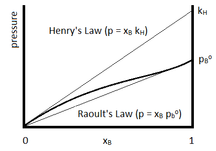
Henry’s Law is depicted by the upper straight line and Raoult’s Law by the lower.
Example \(\PageIndex{1}\): Solubility of Carbon Dioxide in Water
The solubility of \(CO_2(g)\) in water at 25 oC is 3.32 x 10⁻² M with a partial pressure of \(CO_2\) over the solution of 1 bar. Assuming the density of a saturated solution to be 1 kg/L, calculate the Henry’s Law constant for \(CO_2\).
Solution:
In one L of solution, there is 1000 g of water (assuming the mass of CO2 dissolved is negligible.)
\[ (1000 \,g) \left( \dfrac{1\, mol}{18.02\,g} \right) = 55\, mol\, H_2O\]
The solubility of \(CO_2\) can be used to find the number of moles of \(CO_2\) dissolved in 1 L of solution also:
\[ \dfrac{3.32 \times 10^{-2} mol}{L} \cdot 1 \,L = 3.32 \times 10^{-2} mol\, CO_2\]
and so the mol fraction of \(CO_2\) is
\[ \chi_b = \dfrac{3.32 \times 10^{-2} mol}{55.5 \, mol} = 5.98 \times 10^{-4}\]
And so
\[10^5\, Pa = 5.98 \times 10^{-4} k_H\]
or
\[ k_H = 1.67 \times 10^9\, Pa\]
Azeotropes
An azeotrope is defined as the common composition of vapor and liquid when they have the same composition.
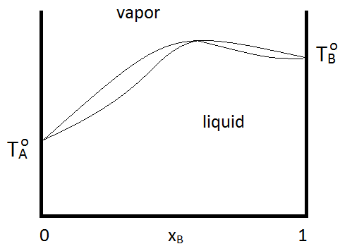
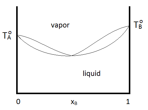
Azeotropes can be either maximum boiling or minimum boiling, as show in Figure \(\PageIndex{2; left}\). Regardless, distillation cannot purify past the azeotrope point, since the vapor and the liquid phases have the same composition. If a system forms a minimum boiling azeotrope and has a range of compositions and temperatures at which two liquid phases exist, the phase diagram might look like Figure \(\PageIndex{2; right}\):
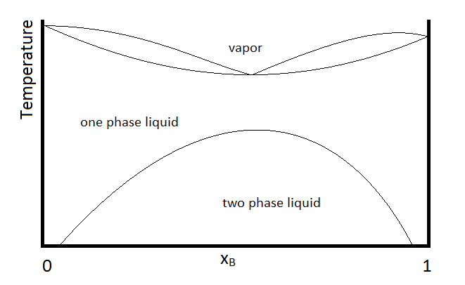
Another possibility that is common is for two substances to form a two-phase liquid, form a minimum boiling azeotrope, but for the azeotrope to boil at a temperature below which the two liquid phases become miscible. In this case, the phase diagram will look like Figure \(\PageIndex{3}\).
Example \(\PageIndex{1}\):
In the diagram, make up of a system in each region is summarized below the diagram. The point e indicates the azeotrope composition and boiling temperature.
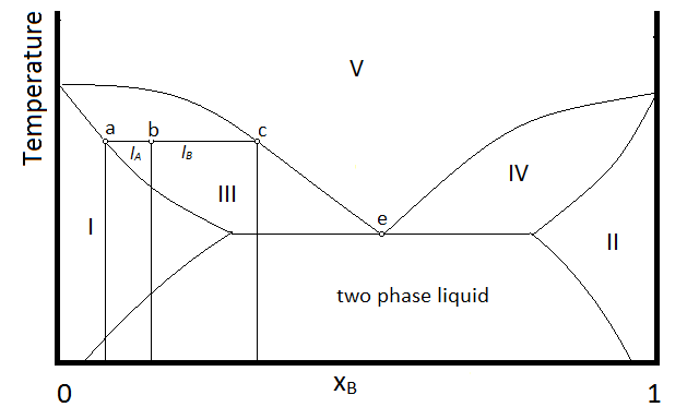
- Single phase liquid (mostly compound A)
- Single phase liquid (mostly compound B)
- Single phase liquid (mostly A) and vapor
- Single phase liquid (mostly B) and vapor
- Vapor (miscible at all mole fractions since it is a gas)
Solution
Within each two-phase region (III, IV, and the two-phase liquid region, the lever rule will apply to describe the composition of each phase present. So, for example, the system with the composition and temperature represented by point b (a single-phase liquid which is mostly compound A, designated by the composition at point a, and vapor with a composition designated by that at point c), will be described by the lever rule using the lengths of tie lines lA and lB.
Gibbs-Duhem and Henry's law
What happens when Raoult does not hold over the whole range? Recall that in a gas:
\[μ_j = μ_j^o + RT \ln \dfrac{P_j}{P^o} \label{B} \]
or
\[μ_j = μ_j^o + RT \ln P_j \nonumber \]
after dropping \(P^o=1\; bar\) out of the notation. Note that numerically this does not matter, since \(P_j\) is now assumed to be dimensionless.
Let's consider \(dμ_1\) at constant temperature:
\[dμ_1 = RT\left(\dfrac{\partial \ln P_1}{ \partial x_1}\right)dx_1 \nonumber \]
likewise:
\[dμ_2 = RT\left(\dfrac{\partial \ln P_2}{ \partial x_2}\right)dx_2 \nonumber \]
If we substitute into the Gibbs-Duhem expression we get:
\[x_1 \left(\dfrac{∂\ln P_1}{ ∂x_1}\right) dx_1+x_2 \left(\dfrac{∂\ln P_2}{∂x_2} \right) dx_2=0 \nonumber \]
Because \(dx_1= -dx_2\):
\[x_ 1 \left( \dfrac{∂\ln P_1}{ ∂x_1} \right) =x_2 \left( \dfrac{∂\ln P_2}{∂x_2} \right) \nonumber \]
(This is an alternative way of writing Gibbs-Duhem).
If in the limit for \(x_1 \rightarrow 1\) Raoult Law holds then
\[P_1 \rightarrow x_1P^*_1 \nonumber \]
Thus:
\[ \dfrac{∂ \ln P_1}{∂x_1} = \dfrac{1}{x_1} \nonumber \]
and
\[\dfrac{x_1}{x_1}=x_2 \dfrac{∂ \ln P_2}{∂x_2} \nonumber \]
\[1=x_2 \dfrac{∂ \ln P_2}{ ∂x_2} \nonumber \]
\[\dfrac{1}{x_2}= \dfrac{∂ \ln P_2}{∂x_2} \label{EqA12} \]
We can integrate Equation \(\ref{EqA12}\) to form a logarithmic impression, but it will have an integration constant:
\[\ln P_2 =\ln x_2 + constant \nonumber \]
This constant of integration can be folded into the logarithm as a multiplicative constant, \(K\)
\[\ln P_2 = \ln \left(K x_2 \right) \nonumber \]
So for \(x_1 \rightarrow 1\) (i.e., \(x_2 \rightarrow 0\)), we get that
\[P_2=K x_2 \nonumber \]
where \(K\) is some constant, but not necessarily \(P^*\). What this shows is that when one component follows Raoult the other must follow Henry and vice versa. (Note that the ideal case is a subset of this case, in that the value of \(K\) then becomes \(P^*\) and the linearity must hold over the whole range.)
Margules Functions
Of course a big drawback of the Henry law is that it only describes what happens at the two extremes of the phase diagram and not in the middle. In cases of moderate non-ideality, it is possible to describe the whole range (at least in good approximation) using a Margules function:
\[P_1= \left(x_1P^*_1 \right)f_{Mar} \nonumber \]
The function \(f_{Mar}\) has the shape:
\[f_{Mar}= \text{exp} \left[ αx_2^2+βx_2^3+δx_2^3 + .... \right] \nonumber \]
Notice that the Margules function involves the mole fraction of the opposite component. It is an exponential with a series expansion. with the constant and linear term missing. As you can see the function has a number of parameters \(α\), \(β\), \(δ\) etc. that need to be determined by experiment. In general, the more the system diverges from ideality, the more parameters you need. Using Gibbs-Duhem is is possible to translate the expression for \(P_1\) into the corresponding one for \(P_2\).