7.5 Introduction to Kinetics
- Page ID
- 218404
\( \newcommand{\vecs}[1]{\overset { \scriptstyle \rightharpoonup} {\mathbf{#1}} } \)
\( \newcommand{\vecd}[1]{\overset{-\!-\!\rightharpoonup}{\vphantom{a}\smash {#1}}} \)
\( \newcommand{\dsum}{\displaystyle\sum\limits} \)
\( \newcommand{\dint}{\displaystyle\int\limits} \)
\( \newcommand{\dlim}{\displaystyle\lim\limits} \)
\( \newcommand{\id}{\mathrm{id}}\) \( \newcommand{\Span}{\mathrm{span}}\)
( \newcommand{\kernel}{\mathrm{null}\,}\) \( \newcommand{\range}{\mathrm{range}\,}\)
\( \newcommand{\RealPart}{\mathrm{Re}}\) \( \newcommand{\ImaginaryPart}{\mathrm{Im}}\)
\( \newcommand{\Argument}{\mathrm{Arg}}\) \( \newcommand{\norm}[1]{\| #1 \|}\)
\( \newcommand{\inner}[2]{\langle #1, #2 \rangle}\)
\( \newcommand{\Span}{\mathrm{span}}\)
\( \newcommand{\id}{\mathrm{id}}\)
\( \newcommand{\Span}{\mathrm{span}}\)
\( \newcommand{\kernel}{\mathrm{null}\,}\)
\( \newcommand{\range}{\mathrm{range}\,}\)
\( \newcommand{\RealPart}{\mathrm{Re}}\)
\( \newcommand{\ImaginaryPart}{\mathrm{Im}}\)
\( \newcommand{\Argument}{\mathrm{Arg}}\)
\( \newcommand{\norm}[1]{\| #1 \|}\)
\( \newcommand{\inner}[2]{\langle #1, #2 \rangle}\)
\( \newcommand{\Span}{\mathrm{span}}\) \( \newcommand{\AA}{\unicode[.8,0]{x212B}}\)
\( \newcommand{\vectorA}[1]{\vec{#1}} % arrow\)
\( \newcommand{\vectorAt}[1]{\vec{\text{#1}}} % arrow\)
\( \newcommand{\vectorB}[1]{\overset { \scriptstyle \rightharpoonup} {\mathbf{#1}} } \)
\( \newcommand{\vectorC}[1]{\textbf{#1}} \)
\( \newcommand{\vectorD}[1]{\overrightarrow{#1}} \)
\( \newcommand{\vectorDt}[1]{\overrightarrow{\text{#1}}} \)
\( \newcommand{\vectE}[1]{\overset{-\!-\!\rightharpoonup}{\vphantom{a}\smash{\mathbf {#1}}}} \)
\( \newcommand{\vecs}[1]{\overset { \scriptstyle \rightharpoonup} {\mathbf{#1}} } \)
\(\newcommand{\longvect}{\overrightarrow}\)
\( \newcommand{\vecd}[1]{\overset{-\!-\!\rightharpoonup}{\vphantom{a}\smash {#1}}} \)
\(\newcommand{\avec}{\mathbf a}\) \(\newcommand{\bvec}{\mathbf b}\) \(\newcommand{\cvec}{\mathbf c}\) \(\newcommand{\dvec}{\mathbf d}\) \(\newcommand{\dtil}{\widetilde{\mathbf d}}\) \(\newcommand{\evec}{\mathbf e}\) \(\newcommand{\fvec}{\mathbf f}\) \(\newcommand{\nvec}{\mathbf n}\) \(\newcommand{\pvec}{\mathbf p}\) \(\newcommand{\qvec}{\mathbf q}\) \(\newcommand{\svec}{\mathbf s}\) \(\newcommand{\tvec}{\mathbf t}\) \(\newcommand{\uvec}{\mathbf u}\) \(\newcommand{\vvec}{\mathbf v}\) \(\newcommand{\wvec}{\mathbf w}\) \(\newcommand{\xvec}{\mathbf x}\) \(\newcommand{\yvec}{\mathbf y}\) \(\newcommand{\zvec}{\mathbf z}\) \(\newcommand{\rvec}{\mathbf r}\) \(\newcommand{\mvec}{\mathbf m}\) \(\newcommand{\zerovec}{\mathbf 0}\) \(\newcommand{\onevec}{\mathbf 1}\) \(\newcommand{\real}{\mathbb R}\) \(\newcommand{\twovec}[2]{\left[\begin{array}{r}#1 \\ #2 \end{array}\right]}\) \(\newcommand{\ctwovec}[2]{\left[\begin{array}{c}#1 \\ #2 \end{array}\right]}\) \(\newcommand{\threevec}[3]{\left[\begin{array}{r}#1 \\ #2 \\ #3 \end{array}\right]}\) \(\newcommand{\cthreevec}[3]{\left[\begin{array}{c}#1 \\ #2 \\ #3 \end{array}\right]}\) \(\newcommand{\fourvec}[4]{\left[\begin{array}{r}#1 \\ #2 \\ #3 \\ #4 \end{array}\right]}\) \(\newcommand{\cfourvec}[4]{\left[\begin{array}{c}#1 \\ #2 \\ #3 \\ #4 \end{array}\right]}\) \(\newcommand{\fivevec}[5]{\left[\begin{array}{r}#1 \\ #2 \\ #3 \\ #4 \\ #5 \\ \end{array}\right]}\) \(\newcommand{\cfivevec}[5]{\left[\begin{array}{c}#1 \\ #2 \\ #3 \\ #4 \\ #5 \\ \end{array}\right]}\) \(\newcommand{\mattwo}[4]{\left[\begin{array}{rr}#1 \amp #2 \\ #3 \amp #4 \\ \end{array}\right]}\) \(\newcommand{\laspan}[1]{\text{Span}\{#1\}}\) \(\newcommand{\bcal}{\cal B}\) \(\newcommand{\ccal}{\cal C}\) \(\newcommand{\scal}{\cal S}\) \(\newcommand{\wcal}{\cal W}\) \(\newcommand{\ecal}{\cal E}\) \(\newcommand{\coords}[2]{\left\{#1\right\}_{#2}}\) \(\newcommand{\gray}[1]{\color{gray}{#1}}\) \(\newcommand{\lgray}[1]{\color{lightgray}{#1}}\) \(\newcommand{\rank}{\operatorname{rank}}\) \(\newcommand{\row}{\text{Row}}\) \(\newcommand{\col}{\text{Col}}\) \(\renewcommand{\row}{\text{Row}}\) \(\newcommand{\nul}{\text{Nul}}\) \(\newcommand{\var}{\text{Var}}\) \(\newcommand{\corr}{\text{corr}}\) \(\newcommand{\len}[1]{\left|#1\right|}\) \(\newcommand{\bbar}{\overline{\bvec}}\) \(\newcommand{\bhat}{\widehat{\bvec}}\) \(\newcommand{\bperp}{\bvec^\perp}\) \(\newcommand{\xhat}{\widehat{\xvec}}\) \(\newcommand{\vhat}{\widehat{\vvec}}\) \(\newcommand{\uhat}{\widehat{\uvec}}\) \(\newcommand{\what}{\widehat{\wvec}}\) \(\newcommand{\Sighat}{\widehat{\Sigma}}\) \(\newcommand{\lt}{<}\) \(\newcommand{\gt}{>}\) \(\newcommand{\amp}{&}\) \(\definecolor{fillinmathshade}{gray}{0.9}\)
Skills to Develop
- To determine the reaction rate of a reaction.
What Happens during a Chemical Reaction?
A chemical reaction occurs when atoms in existing substances are rearranged and recombined to form new substances. The reaction is similar to taking apart a Lego structure that currently exists and using the small pieces to make a new structure. In most chemical reactions existing bonds are broken and new bonds are formed. Not all chemical reactions involve both bond breaking and bond making, but the vast majority of reactions do. Energy is always required to break a bond and energy is always given off when a bond is made.
Note
Bond breaking always requires the input of energy. Bond formation always gives off energy. No exceptions to these facts!
Thus, to start a chemical reaction, you must almost always put some energy into the chemicals so that you can break the bonds in the reactant particles. The minimum amount of energy required to break the existing bonds is called the activation energy, and it is given the symbol Ea. If the particles are moving fast enough, they will have a large enough kinetic energy so that some or all of the bonds in the particles will break when the particles collide with each other. But simply colliding with enough energy to break the existing bonds is not enough to get a reaction to occur. It turns out that the particle have to be in just the right position when they collide together for the bonds to break. An analogy for the need for the proper orientation of the particles is throwing darts at a dart board. If a dart is thrown sideways at a dart board, it will not stick in the board, even if you throw it with a lot of energy. Likewise, molecules can run into each other at very high speeds, but if they don't collide when facing the right way, no bonds will break and there won't be a reaction. In summary, to get an effective collision between particles, the particles need to have
1. sufficient energy (the activation energy)
2. proper orientation.
Keeping this description of a chemical reaction in mind, let's see what happens to the amount of reactants and the amount of products as a reaction occurs.
Reaction Rates
Reaction rates are usually expressed as the concentration of reactant consumed or the concentration of product formed per unit time. The units are thus moles per liter per unit time, written as M/s, M/min, or M/h. To measure reaction rates, chemists start the reaction, measure the concentration of the reactant or product at different times as the reaction progresses, perhaps plot the concentration as a function of time on a graph, and then calculate the change in the concentration per unit time.

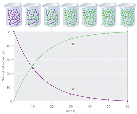
Figure \(\PageIndex{1}\): The Progress of a Simple Reaction (A → B). The mixture initially contains only A molecules (purple). Over time, the number of A molecules decreases and more B molecules (green) are formed (top). The graph shows the change in the number of A and B molecules in the reaction as a function of time over a 1 min period (bottom).
The progress of a simple reaction (A → B) is shown in Figure \(\PageIndex{1}\); the beakers are snapshots of the composition of the solution at 10 s intervals. The number of molecules of reactant (A) and product (B) are plotted as a function of time in the graph. Each point in the graph corresponds to one beaker in Figure \(\PageIndex{1}\). The reaction rate is the change in the concentration of either the reactant or the product over a period of time. The concentration of A decreases with time, while the concentration of B increases with time.
\[\textrm{rate}=\dfrac{\Delta [\textrm B]}{\Delta t}=-\dfrac{\Delta [\textrm A]}{\Delta t} \label{Eq1}\]
Square brackets indicate molar concentrations, and the capital Greek delta (Δ) means “change in.” Because chemists follow the convention of expressing all reaction rates as positive numbers, however, a negative sign is inserted in front of Δ[A]/Δt to convert that expression to a positive number. The reaction rate calculated for the reaction A → B using Equation \(\ref{Eq1}\) is different for each interval (this is not true for every reaction, as shown below). A greater change occurs in [A] and [B] during the first 10 s interval, for example, than during the last, meaning that the reaction rate is greatest at first.
Reaction rates generally decrease with time as reactant concentrations decrease.
Determining the Reaction Rate of Hydrolysis of Aspirin
We can use Equation \(\ref{Eq1}\) to determine the reaction rate of hydrolysis of aspirin, probably the most commonly used drug in the world (more than 25,000,000 kg are produced annually worldwide). Aspirin (acetylsalicylic acid) reacts with water (such as water in body fluids) to give salicylic acid and acetic acid, as shown in Figure \(\PageIndex{2}\).

Figure \(\PageIndex{2}\): Hydrolysis of Aspirin reaction.
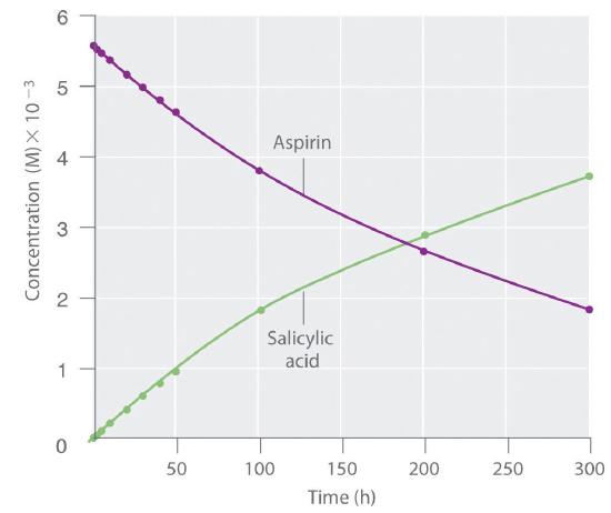
Because salicylic acid is the actual substance that relieves pain and reduces fever and inflammation, a great deal of research has focused on understanding this reaction and the factors that affect its rate. Data for the hydrolysis of a sample of aspirin are in Table \(\PageIndex{1}\) and are shown in the graph in Figure \(\PageIndex{3}\).
| Time (h) | [Aspirin] (M) | [Salicylic Acid] (M) |
|---|---|---|
| *The reaction at pH 7.0 is very slow. It is much faster under acidic conditions, such as those found in the stomach. | ||
| 0 | 5.55 × 10⁻³ | 0 |
| 2.0 | 5.51 × 10⁻³ | 0.040 × 10⁻³ |
| 5.0 | 5.45 × 10⁻³ | 0.10 × 10⁻³ |
| 10 | 5.35 × 10⁻³ | 0.20 × 10⁻³ |
| 20 | 5.15 × 10⁻³ | 0.40 × 10⁻³ |
| 30 | 4.96 × 10⁻³ | 0.59 × 10⁻³ |
| 40 | 4.78 × 10⁻³ | 0.77 × 10⁻³ |
| 50 | 4.61 × 10⁻³ | 0.94 × 10⁻³ |
| 100 | 3.83 × 10⁻³ | 1.72 × 10⁻³ |
| 200 | 2.64 × 10⁻³ | 2.91 × 10⁻³ |
| 300 | 1.82 × 10⁻³ | 3.73 × 10⁻³ |
The data in Table \(\PageIndex{1}\) were obtained by removing samples of the reaction mixture at the indicated times and analyzing them for the concentrations of the reactant (aspirin) and one of the products (salicylic acid).

Figure \(\PageIndex{3}\): The Hydrolysis of Aspirin. This graph shows the concentrations of aspirin and salicylic acid as a function of time, based on the hydrolysis data in Table 14.1. The time dependence of the concentration of the other product, acetate, is not shown, but based on the stoichiometry of the reaction, it is identical to the data for salicylic acid.
In the next section, we will look at how we can affect the reaction rate.

