4.5: Writing a Method for the Agilent 1100/1200 HPLC

A method is a list of steps that control the components of the instrument and create the chromatographic conditions required to perform an analysis. The instructions that follow are designed to set up a method for Part 1 of the HPLC experiment.

Writing an isocratic method

1. Select Load Method from the Method menu, and then choose default.M from the list of methods.

Figure \(\PageIndex{1}\): The Setup Method dialog box, on the Binary Pump Tab.

2. You will now edit the default method. Select Edit Entire Method from the Method menu.
3. In the Edit Method box that appears, click on OK to continue. (Note: If you wish to discontinue editing at any time, select CANCEL.)

   

   Figure \(\PageIndex{2}\): The Edit Method dialog box. Select all options and press OK.

4. The Method Information dialog box will appear. Move the cursor to the Method Comments text area and click on the left mouse button. Enter information about the method, for example: 60% METHANOL/40% WATER AT 1.000 ml/min. Select OK to continue.
5. In the Injection Source/Location, accept the default, HipAls, which is the automatic sample injector. Press OK.
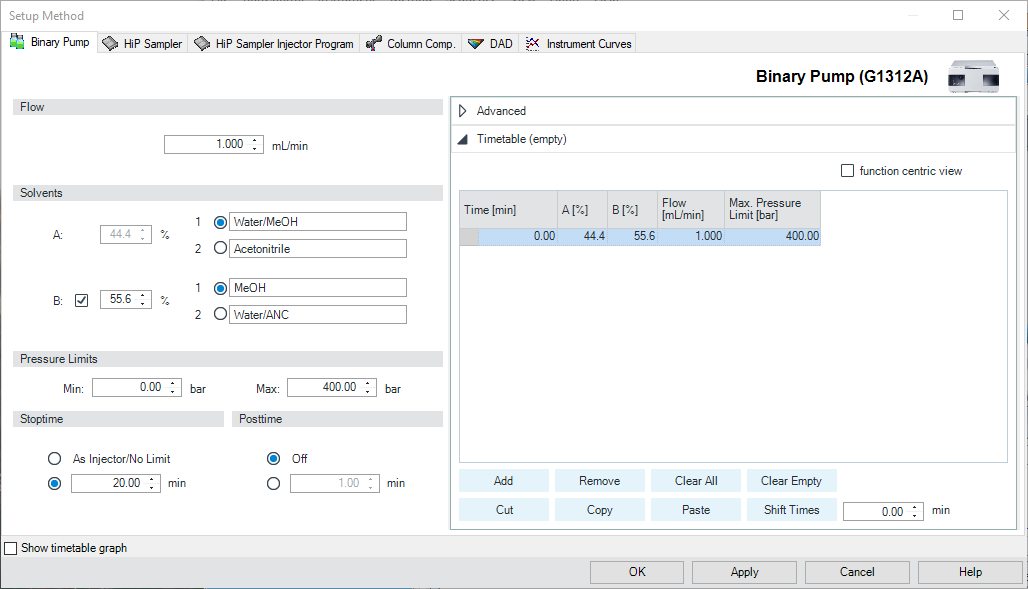
6. In the Setup Method Box, go to the Binary Pump tab (Figure \(\PageIndex{2}\)). Check that the Flow is set to 1.000 ml/min. This flow rate will be used during all subsequent experiments, unless specific contrary instructions are given.
7. The StopTime (length of the analysis) should be 5 minutes. The PostTime need not be used. (Figure \(\PageIndex{2}\))
8. Now check the mobile phase composition to be used. In this experiment, you will use solvents A1 (water), B1 (methanol). Enter the solvent composition 60/40 B1/A1. (Figure \(\PageIndex{1}\))
9. The default pressure limits of 0 - 400 bar is appropriate for this entire experiment, and do not need to be changed. If the Min and Max pressure limits differ from these default values, they should be reset to 0 and 400 bar, respectively. (Figure \(\PageIndex{2}\))
10. This will be an isocratic (constant mobile phase composition) analysis, and you do not need to modify the Timetable editor; the timetable is customized only for gradient runs. Delete any text that appears in the Timetable box other than the first line that sets initial conditions at time zero. (Figure \(\PageIndex{2}\)).
11. Go to the HiP Sampler Tab (Figure \(\PageIndex{3}\)). Check that the injection volume is 5.00 µl. The other parameters should be left unchanged at the default values.

    

    Figure \(\PageIndex{3}\): The Setup Method dialog box, on the HiP Sampler Tab.

12. Go to the Column Components (Column Comp.) tab (Figure \(\PageIndex{4}\)). Select Not Controlled for both Left and Right temperature controls.

    

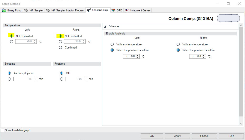
    Figure \(\PageIndex{4}\): The Setup Method dialog box, on the Column Comp. Tab.

13. Go to the Diode Array Detector (DAD) tab (Figure \(\PageIndex{5}\)). The DAD detector is used to monitor absorption of UV-vis light as analytes elute from the column.
    • Set Signal A, B, and C to 254, 280 and 310 nm respectively.
    • Check the box under "Acquire" to activate each signal, and enter the appropriate wavelength in the box.
    • The default bandwidths of 4 nm need not be changed.
    • All reference wavelengths should be set to OFF by leaving the Reference Wavelength box unchecked.
    • All other parameters may be left at the default values.

      Figure Figure \(\PageIndex{5}\): The Setup Method dialog box, on the DAD Tab.

14. Click OK at the bottom of the Setup Method box.
15. The Signal Details dialog box will appear. Choose signals A, B, and C and press the Add to Method button to add each of the available signals to the method. Then Press OK.

    

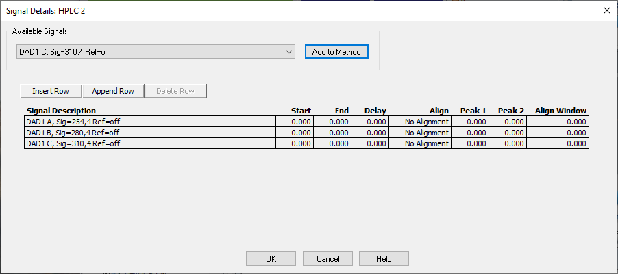
    Figure \(\PageIndex{6}\): Signal Details box.

16. The Integration Events dialog box allows you to control how a chromatogram is integrated. Click on the icon with a green check mark. Then, make sure the values match those shown here.

    

    Figure \(\PageIndex{7}\): Integration Events box.

17. The Specify Report dialog box allows you to specify how the results should be reported. You will generate, and print, a chromatogram and an Area Percent report with calculations based on area and sorted by retention time. The raw data will be stored in a file and sent to the printer. Click OK to continue.

    

    Figure \(\PageIndex{8}\): Specify Report box.

18. In the Instrument Curves dialog box, no options are selected. Click OK to continue.

    

    Figure \(\PageIndex{9}\): Instrument Curves box.

19. Select only the Data Acquisition and Standard Data Analysis method sections in the Run Time Checklist dialog box and select OK to continue.

    

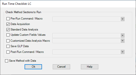
    Figure \(\PageIndex{10}\): Run Time Checklist box

20. Select Save Method As from the Method menu. When the Save Method As box appears, type a name for the method file (eg yourinitials_ic_40A60B.m) in the text box. Click on OK to save the method. There is no need to put anything in the Comment for Method History box.

Writing a gradient method

To write a gradient method, you can follow all the same steps as described above for an isocratic method; however, you would adjust the Timetimble options in the Binary Pump tab of the Edit Method dialog box. When writing a gradient method, these are the major steps Dr. Haas recommends:

1. Pre-gradient elution step - flow one column volume (void volume) of solvent at the starting condition through the column. This ensures that the sample is loaded onto the column under the starting conditions.
2. Gradient - run the gradient from weak to strong solvent composition. A typical gradient is to start at 97%A/3%B and end at 3%A/97%B.
3. Post-gradient elution - flow one column volume of the strong solvent condition through the column.
4. Post-gradient equilibration - this step sets you up for the next run. It is optional to build it into your method, and it only makes sense if the next injection will occur under the same starting conditions as this run. Return the condition to the starting sovent composition (weak solvent) and run for at least 5, and ideally 10 column volumes.

An example of a gradient table is shown below in Figure \(\PageIndex{11}\), where the option to Shot timetable graph is also selected.

Figure \(\PageIndex{11}\): Setup Method box with an example of a gradient timetable.