2.6: Procedure and instructions for data analysis

The main objective of this in-lab module is to practice using volumetric equiptment correctly, and to use data to self-assess your ability to create solutions with high precision. To do this, you will use a colored dye that absorbs light in the visible region of the electromagnetic spectrum.

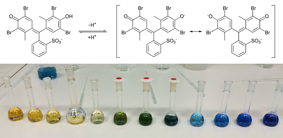
Bromocresol green

Bromocresol green (pKa = 4.66) is an acid-base indicator dye that exhibits a pH-dependent absorption spectrum. The only structural difference between the acid form (yellow) and the basic form (blue) of this dye is the protonation of a phenolic oxygen. This experiment will be performed in 0.01 M sodium acetate; the presence of this weak base in solution will ensure that the the bromocresol green dye is predominantly in its basic form.

You will be given a stock solution of bromocresol green. You will use this stock solution to prepare a series of more dilute solutions. You will measure the absorbance of the diluted solutions at 612 nm (absorption maximum for the basic form of the dye) and generate a calibration curve of absorbance vs concentration. You will then measure the absorbance of a bromocresol green solution of unknown concentration, and use Beer's law to determine its concentration.

Figure \(\PageIndex{1}\): Top: acid dissociation of bromocresol green. Bottom, from left to right: five solutions of 0.1 M HCl with decreasing concentrations of bromocresol green (yellow); three buffered solutions at pH 3.78, pH 4.00, and pH 4.62 (shades of green) and four solutions of NaOH 0.1 M with increasing concentrations of bromocresol green (darker solutions are more concentrated). (Natan Consigli, Bromocresolo, crop, CC BY-SA 4.0)

Materials

Gather the following:

• \(5.00 \times 10^{-4}\) M bromocresol green stock solution in 0.1M sodium acetate (prepared by the TA in advance by dissolving 0.0900 g of the sodium salt of bromocresol green (MW 720.02 g/mol) and 0.3402 g of sodium acetate trihydrate in 250.00 ml of DI water). The exact concentration should be written on the stock container. This is the stock solution.
• "Control" solution of known concentration. This is a solution of bromocresol green in 0.1 M sodium acetate. You will use this solution to test your standard curve. The exact concentration should be written on the control solution storage container.
• "Unknown" solution (a solution of bromocresol green of unknown concentration).
• 125 mL of 0.01 M sodium acetate: Prepared by the TA in advance by dissolving 2.7216 g of sodium acetate trihydrate (MW 136.08 g/mol) in 2.00 L of deionized water.
• One 1000 µL automatic pipette (you will share with other students)
• One 15 ml volumetric pipette
• At least one 25 ml volumetric flasks (you could use up to five if available)
• One disposable transfer pipet
• Two glass cuvettes
• Spec 20 instrument
• One beaker to collect waste

Procedure

Table \(\PageIndex{1}\): Example table for recoding data on calibration standards. All samples are diluted with 0.01 M Sodium acetate solution.

Trial 1 data			Replicate measurements of absorbance (AU)
Solution Label	Components	Concentration of Bromocresol	1	2	3	Average Absorbance (with error)
A (Stock solution, ~\(5.00 \times 10^{-4}\))	Stock solution of Bromocresol Green (undiluted)		NA	NA	NA
B	1.000 mL of stock, diluted to 25.00 mL
C	15.00 mL B, diluted to 25.00 mL
D	15.00 mL C, diluted to 25.00 mL
E	15.00 mL D, diluted to 25.00 mL
F	15.00 mL E, diluted to 25.00 mL
Blank	0.01 M sodium acetate	0

Create a serial dilution

You will make a series of sequential or "serial" dilutions of bromocresol green and measure the absorbance of each solutions in the series using a Genesys 20 spectrometer. You will use these data to construct a calibration curve and determine the concentration of an "unknown" solution.

1. Create the serial dilutions:Using a 1 ml automatic pipette, quantitatively transfer 1.000 ml of stock solution to a 25 ml volumetric flask. Carefully dilute the solution up to the mark using 0.01 M sodium acetate solution. This is solution B (see table). Put some of this solution into a screw cap vial labeled "B" so that you can access the solution with a pipette in the next step. You can also store the leftover solution B in this vial.
   • Using a 15 ml volumetric pipette, quantitatively transfer 15 ml of solution B to a clean 25 ml volumetric flask. Carefully dilute the solution up to the mark using 0.01 M sodium acetate solution. This is solution C. If you are re-using your 25 mL flask for the next solution, transfer solution C to a labeled vial before the next step. 
   • In the same manner, perform 3 more serial dilutions according to Table 1. Transfer each solution to a labeled vial and keep vials closed to avoid evaporation.
2. Calculate the concentration of bromocresol green in each solution. (Remember: \(M_1V_1=M_2V_2\).) Also calculate the error associated with each solution's concentration using error propagation.

Data Collection

Measure and record the absorbance of each solution at 612 nm using a Spec 20. You should measure the concentration of each solution in the serial dilution, the control, and the unknown. Instructions for operating the Spec 20 are in the section, Operating Instructions for Spec 20 Visible Spectrometers.

Tips for data collection

• Use one cuvette for all measurements and keep a second separate cuvette for all blanks. The blank cuvette should be filled with 0.01 M sodium acetate solution.
  **Its a good idea to make sure that both cuvettes yeld zero absorbance with the sodium acetate solution in both after the instrument is zeroed with one of them.
• Work starting with the least concentrated solution and proceed in order of increasing concentration.
• The outside of the cuvette should always be clean and dry.
• Take three measurements for each solution (use same liquid for each measurement; take cuvette out and wipe down then replace in instrument) and calculate the average absorbance and standard deviation from three readings for each solution. Usually, you should get exactly the same absorbance reading for all three replicate measurements. The three readings should not differ by more than \(\pm 0.003\) absorbance units or 1% of the absorbance (see uncertainty associated with the spectrometer readings described in the operating instructions.)
• Between each measurement, the sample cuvette should emptied and then rinsed twice with small (ca. 1 mL or less) aliquots of the next solution to be assayed.
  ***Work carefully because you have limited quantities of each solution.
• Between measurements, check the stability of the instrument by inserting the blank and making sure it still reads zero absorbance.

Procedure for data collection 

1. Blank the Spec 20 using a cuvette filled with 0.01M sodium acetate. Keep this cuvette filled with sodium acetate for future use.
2. Fill a second cuvette with 0.01 M sodium acetate and measure its absorbance to be sure the second cuvette matches the first. The reading should be very close to zero.
3. Measure and record the absorbances of each solution in the serial dilution.
4. Measure and record the absorbance of the "control" solution.
5. Measure and record the absorbance of the "unknown" solution.
6. Keep your solutions until you have validated your calibration curve and determined that you do not need to repeat any of the absorbance readings.

Treatment of data

Specific expectations for this module are given below. You may use any data analysis software you wish. We recommend you use Excel, using a calibration template as described in previously in this module. Alternatively, you could use Matlab (and the lsq custom script) or LoggerPro to do this analysis.

1. Prepare a table of absorbance vs solution concentration (similar to Table \(\PageIndex{1}\)).
   • At zero concentration of bromocresol green, you had zero absorbance (the blank). Therefore, you should also have the point (0, 0) in your data table (or whatever absorbance you measured at zero concentration).
   • Include error in the value of each concentration (determined using error propagation; see info above on how stock was created).
   • Include the error associated with your absorbance readings. This should be the same as the tolerance of the instrument or the standard deviation of the three replicate measurements; whichever is greater.

     Important Note

     If the standard deviation of the replicate absorbances is much greater than the uncertainty expected for the instrument (see operating instructions), there may be a technical issue with data collection!

     ​​​​
2. Plot the standard (calibration) curve of absorbance vs concentration. The following points will always be expected in this course!
   • Plot instrument response (in this case, absorbance) vs concentration of the serial dilution solutions in scatter format (not line).
   • Maximize the area occupied by data by adjusting scales of X and Y axes.
   • Perform a least squares analysis (lsq in Matlab or LINEST in Excel) of all six data points for your standard curve. Plot the best-fit line on the plot. Report the equation for the best fit line on your plot (including the error determined by lsq).  Report error in the y-intercept and slope. **Note that slope is the response factor.
   • Label both axes with units.
   • Give a descriptive at the top of the figure. (eg "Standard curve: Absorbance at 612 nm vs concentration of bromocresol green at pH ~10.")
   • Give a figure number and a descriptive caption under the figure. (eg "Figure 1. Bromocresol green at pH 10 shows a maximum absorbance at 612 nm. The absorbance of the solution increases with concentration. The dependence of absorbance on concentration is shown for solutions of bromocresol green dissolved in 0.01 M sodium acetate.")
   •  
3. State the response factor (aka molar absorptivity (\(\epsilon\))) of Bromocresol Green at 612 nm under the conditions used here. Report the value (with associated error) from your standard curve (it is the slope). Do not just simply rely on your labeled plot. Use a short statement to report the response factor and state whether the response fits well to a straight line.
   *Recall Beer's law gives the relation between the absorbance (A) of a solution and the solution concentration (c (in moles/liter)): \[A = \epsilon b c\]​​​​where \(\epsilon\) is the molar absorptivity (L cm-1 mol-1), and b is the path length of the light passing through the solution (width of the cuvette). Though you could calculate this from each point on your plot, do not. Please use the slope of your line.
4. Validate your calibration curve using the control solution. Use the your calibration to calculate the concentration of bromocresol green in the control solution. Report the experimental concentration together with the associated uncertainty. 
   • Determine error in the determined value and show the equation used. Even though you probably did this using your excel template, show the equation in the document you turn in!
   • Compare the experimentally-determined concentration of the control solution to the known concentration. Are the two values the same? If they are not exactly the same, are they essentially equal considering the estimated error in each value?
     • It is up to you to determine if the value you found for the control solution is accurate within experimental error before leaving lab for the day.
     • If the value you determined is different from the actual control solution concentration, it is a sign that there may be an issue with the preparation of the serial dilution or with the collection of data. You should consult with your TA and/or your Professor to troubleshoot and determine the most likely source of error so that you can fix any problems before repeating the calibration - the goal is to learn the correct techniques before you repeat the entire procedure.
     • Proceed to the next step only after you have validated your calibration curve.
5. Use your validated standard curve to calculate the concentration of bromocresol green in the unknown solution. Report the experimental concentration together with the associated uncertainty.

All steps above, including data analysis should be completed in the first lab period; this is so that you can take advantage of your instructors to help you troubleshoot as necessary. Students who wish to repeat the procedure above in the next lab period may do so to improve their technique; good technique will be critical for performance in the rest of this course.

Complete all data analysis before the end of the second laboratory meeting of the semester; the results should be checked by your TA and also submitted on Gradescope. See Gradescope for a rubric on this assignment!

Shut down\cleanup

Only when you are absolutely sure that you are finished for the day, please do the following shut-down and cleaning tasks:

• Store solutions for next week if necessary.
• Bromocresol green and sodium acetate waste should go in the labeled waste container in the hood dedicated for waste. Do not overfill the waste - notify a TA if the waste is above the shoulder of the bottle (where the bottle begins to narrow).
• Volumetric pipetes should be rinsed with deionized water to remove excess reagent solution, and then placed in the pipete washer with tips UP (toward the ceiling). The pipete washer is a huge white plastic tube with a screen at one end. It will be in the sink near the drawers where the pipettes are stored.
• Rinse all other glassware 3 times with deionized water and remove all labels. Dry the glassware as well as possible and return it its storage location.
• Check the sink and other areas where you worked to be sure you did not leave anything lying around.
• Replace all automatic pipetters to their racks and place the tips nearby.
• Wipe down the bench and sink area with a damp paper towel.

Sources:

1. Skoog, D. A.; West, D. M.; Holler, F. J. Fundamentals of Analytical Chemistry, 7th edition, Saunders College Publishing, 1996.

2. Pickering, M. and Heiler, D. J. Chem. Ed., 1987, 64(1), 81.