Perform the tasks listed here using the instructions for using Hulis that are given below.
Perform HMO calculations for each of the four dyes. In the HMO analysis, omit the ethyl groups since they are not part of the conjugated network. Save a screen-shot image of the entire program window showing the structure and the orbital diagram before moving on to the next one.
Calculate the energy difference, ∆E, between the HOMO and LUMO levels (in terms of \( \beta \)) for each dye.
Plot the HMO ∆E's (abscissa) versus the experimentally observed ∆E's (kJ/mol) (from step (4) above) (ordinate). From the least-squares slope of the resultant line, determine a semiempirical value for the spectroscopic \( \beta \). Compare your value with the accepted range for the spectroscopic exchange integral, – 250 to – 350 kJ/mole.9 Report the uncertainty in \( \beta \).
Use your value of \( \beta \) to calculate the energy difference, ∆E, between the HOMO and LUMO levels in units of kJ/mol and eV for each dye. Using these energies, calculate the wavelength (nm) at which you would expect to observe this HOMO \( \rightarrow \) LUMO transition for each dye, using the HMO model.
Calculate the percent error between your calculated HMO results your experimental values. Tabulate your data in the format shown below.
WAVELENGTH (nm)
Dye #
\( \lambda_{max} \)
Literature*
\( \lambda_{max} \) Experimental
\( \lambda_{max} \) Particle-in-box
\( \lambda_{max} \) HMO
Value (nm)
Absolute Error (nm)
Value (nm)
% Error
(from exp.)
Value (nm)
% Error
(from exp.)
±
±
±
±
* reference for your literature values goes here
Use this table as the basis for discussion of your results. Which theoretical model gives the best fit to the experimental data, and why? Are the results for each dye equally satisfactory? If your answer is no, explain why you think this is so. How are these models useful and what might be done to improve the results?
Calculate the wavelength (nm) and minimum excitation energy (eV) of the molecule CH2=CHCH=CHCH=CHCH=CH2 using the HMO model program. In calculation use your value of \( \beta \) to convert to electron volts. What color does the molecule absorb from white light? What color does it then appear?
Instructions For Using The Program "Hulis" ver. 3.0.x
Note
Hulis is a Java applet. Java must be installed to run the applet. You are welcome to run it from your own laptop if Java is installed. But for your convenience in the event that you do not want Java on your computer, the program is available on all of the lab computers.
Double-click on the Hulis icon to Start the Program
Running the Program:
The main screen shows a molecule builder. Highlight Build on the left side of the screen if it is not already highlighted when the program starts.
Figure \(\PageIndex{1}\): The Hulis Main Screen. (CC-NC-BY-DUKE CHEM)
To build a molecule, for example, Dye 1, begin by clicking anywhere in the blank window in the center of the screen. A CH3 group should appear. Click on one of the available hydrogens to add a conjugated carbon to your molecule. As you add carbons to form the first ring, you will see the orbital diagram for the molecule appear in the right-hand panel of the program.
You can follow the electron count from this pane of the program window. After putting 6 carbons to form the ring, you will need to form a bond between the two open and adjacent carbons. To do this, simply click on one of the open carbons and drag a bond over to the adjacent open carbon. The hydrogens will disappear and a delocalized C-C bond will form.
Continue adding carbon atoms as appropriate to form the template molecule. When you are done your structure will look like this:
Figure \(\PageIndex{2}\): Dye 1. Note that for the purposes of a Hückel calculation the ethyl groups are omitted (CC-NC-BY-DUKE CHEM)
Note
You can rescale the display on the screen using Zoom out from the Display menu. You can also move, rotate, and center the molecule in the display window with the appropriate control buttons in the left-hand (blue colored) pane of the program window. In the image above the Move button is currently highlighted.
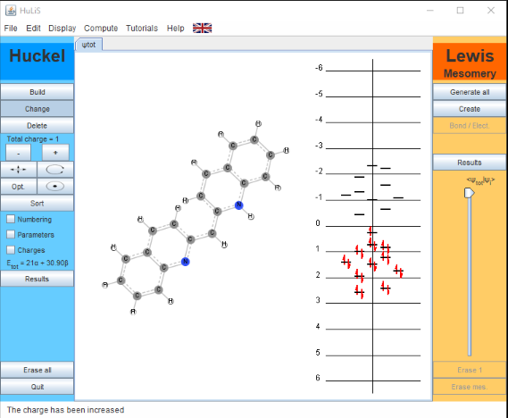
You now need to change two of the carbon atoms to nitrogen to complete the structure. Click on the Change button in the left-hand pane, and then double-click on the appropriate carbon in your structure. A Change Atom box appears. Select =NR to change this to the pyridinium group. Check to be sure the value in the Hx box = 0.51. Click on OK. Now change the other carbon to a nitrogen in the same way, but this time select the –NR2 option. Be Sure the value in the Hx box = 1.37. Click OK. Finally, make the molecule a cation by clickingh the + in the left-hand pane to increase the Total charge to 1. You final molecule will look as shown below.
Figure \(\PageIndex{3}\): 1,1'-Diethyl-2,2'-Cyanine Iodide. The ethyl groups are omitted to simplify the calculations. (CC-NC-BY-DUKE CHEM)
Looking at the orbital diagram in the right-hand (orange) pane of the program screen you will see the occupied and unoccupied orbitals, as calculated by the simple Hückel approximation. You can see that the 21 pi-electrons in the molecule occupy the first 11 pi-orbitals; the HOMO to LUMO transition occurs between the 11th and 12th pi-orbital.
Click on the Results button, and a Results window appears with significant information about the Hückel calculation. Please note the following things:
As you scan down the Hamiltonian matrix check to see that the Coulomb and Exchange integrals for heteroatoms and carbon-to-heteroatom bonds are as shown in the table below. If you need to see how your atoms are numbered in your structure to make it easier to find them in the Result table, put a check in the Numbering box in the left hand pane of the program window.
Atom
Bond
Number of
p-Electrons
Coulomb
Integral
Exchange
Integral
C
1
0.00
1.00
N
Pyridine
2
1.37
0.89
N
Pyridinium
1
0.51
1.02
In the Orbitals section of the Results box count over the appropriate number of orbitals (11 in the case of Dye 1), and record the results for the HOMO and LUMO in this molecule.
Figure \(\PageIndex{4}\): Orbital Energies for Dye 1. (CC-NC-BY-DUKE CHEM)
Notice that in this case the energy of the HOMO is \( \alpha + 0.2737 \beta \); and, the energy of the LUMO is \( \alpha -0.4390 \beta \).
Note
NOTE: you can change the number of digits in the display from Preferences, under the File menu.
Close the Results Box.
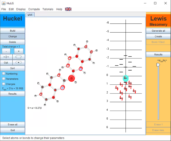
To get a visual representation of the pi-molecular orbitals generated in the Hückel program, simply click on one of the orbitals in the right-hand pane of the program window. The orbital will appear on top of the molecule in the main screen. The image below is of the HOMO.
You can turn off the orbital display from your molecule by clicking below the orbitals in the right-hand pane of the program window. Save a screen-shot image of the entire program window showing the structure and the orbital diagram.
Figure \(\PageIndex{5}\): The Highest Occupied Molecular Orbital in Dye 1. (CC-NC-BY-DUKE CHEM)


You now need to change two of the carbon atoms to nitrogen to complete the structure. Click on the Change button in the left-hand pane, and then double-click on the appropriate carbon in your structure. A Change Atom box appears. Select =NR to change this to the pyridinium group. Check to be sure the value in the Hx box = 0.51. Click on OK. Now change the other carbon to a nitrogen in the same way, but this time select the –NR2 option. Be Sure the value in the Hx box = 1.37. Click OK. Finally, make the molecule a cation by clickingh the + in the left-hand pane to increase the Total charge to 1. You final molecule will look as shown below.