9.7: Exercise 4 - Modeling the Absorption Spectrum of Cyanine Dyes

 

This experiment is designed to build and study the series of conjugated dyes used in the UV-Vis experiment earlier in the course. For reference, the substitution number of napthalene is shown in the figure below (from Wikipedia).

Figure \(\PageIndex{1}\): Numbering of the carbon atoms in naphthalene molecules according to latest (2013) IUPAC rules P-25.3.2.3 and P-25.3.3.1, which is the same as 1979 rule A-22. (By User:Edgar181 - Own work, Public Domain, https://commons.wikimedia.org/w/inde...curid=22671537)

1. The first dye you will build and work with is the 1,1’-diethyl-4,4’-carbocyanine cation. (See Figure 3.2.2 in Experiment 1). Start a new file. Select the Inorganic tab of the Builder. Under Rings select Naphthalene. Click in the workspace to place a naphthalene ring on the screen. Now select the sp² hybridization option and check to see that the element in the element selection button is Carbon. Move to the working area and add three sp² carbons to the 1-position of the naphthylene ring. At this point your structure should look something like this.

Figure \(\PageIndex{1}\): Adding \(sp^2\) Carbons to the Naphthalene Ring. (CC-NC-BY-DUKE CHEM)

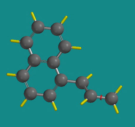
Return to the Naphthalene selection under Rings again. Notice the small yellow circle on the structure in the Rings window . This indicates the “active” valence of the naphthyl group. Make the 1-position of naphthyl active by clicking on the valence in the small structure window. Click on the free valence of the 3^rd carbon atom in the working area, to add the second ring to your structure. At this point it might look something like this.

Figure \(\PageIndex{2}\): Adding the Second Naphthalene Ring. (CC-NC-BY-DUKE CHEM)

Now click on the delocalized bond . Double click on each C–C bond connecting the three carbons to each other and to the two rings. Look closely to be sure that all C–C bonds are delocalized.

Figure \(\PageIndex{3}\): Changing the Bond Order of the Connecting Carbons. (CC-NC-BY-DUKE CHEM)

Click on the button to minimize the structure. Chances are good that not all of the connecting carbons between the rings are in the trans- orientation, and that the overall structure is not yet planar. You can rotate around specific bonds to alter the conformation of the molecule. To do this, click on a bond you wish to rotate around. A red arrow appears, wrapping around the bond.

Figure \(\PageIndex{4}\): The Rotate Fragment Arrow. (CC-NC-BY-DUKE CHEM)

Hold down both the control and shift keys and click and drag the left mouse button to rotate a fragment of the molecule around the selected bond. In this way put all of the connecting carbons into the trans-orientation, and position the rings so that they point up and outward away from each other. Click again on the button to minimize the structure. It should now be planar and look like this.

Figure \(\PageIndex{5}\): The Nearly Completed Structure. (CC-NC-BY-DUKE CHEM)

Return to the element section button and choose Nitrogen. Double-click on the carbon atoms of the naphthalene rings that are para- (across from, and in position 4) to the connecting three-carbon chain (look ahead to Figure \(\PageIndex{6}\)). The color of the atom should change to blue as the element changes from carbon to nitrogen. Change the element selection button back to Carbon, and change the hybridization to sp³ . Add ethyl groups to the free valence of the nitrogen atoms. Minimize the structure using . Check your structure. Is it planar? The final molecule should look something like this (rotated some to show the planar nature).

Figure \(\PageIndex{6}\): The Completed Structure. (CC-NC-BY-DUKE CHEM)

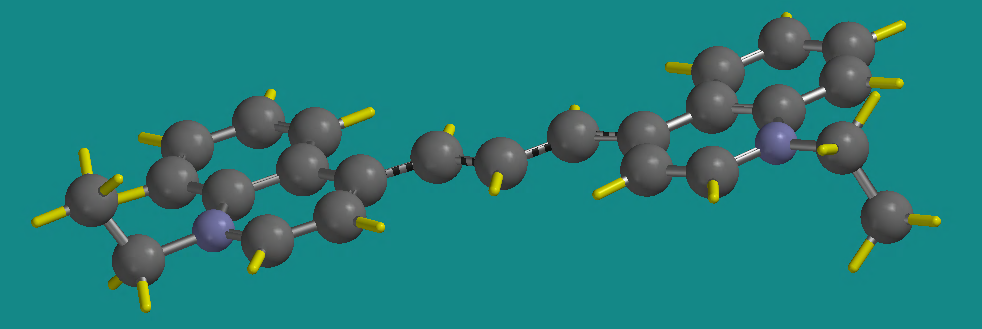
Notice in this picture that the ethyl groups are positioned axial to the plane of the rings. Save this molecule as dye4.

2. At this point you might see that it take more work to build a larger molecule. It might be prudent, therefore to keep the dye4 file safe, just in case something happens and you need to recall it. To do so, select Save as from the File menu and save the file as dye4_MNDO. Select Setup, Calculations from the menu. Choose calculate: Equilibrium Geometry at Ground State in Gas with Semi-Empirical, MNDO. Set Total charge : Cation, Unpaired Electrons: 0. Click Submit.

3. Once the calculation is finished, inspect the molecule. Did the conformation change? Inspect the Output and record the equilibrium geometry Energy from the Summary section in your lab notebook.

4. In preparation for the next calculation select Save As from the File menu and name the file dye4-ci. Then select Setup, Calculations again, and change the parameters to, Calculate: Energy at Ground State in Gas with Semi-Empirical, MNDO. Set Total charge : Cation, Unpaired Electrons: 0. In the Options box: type CI PRINTLEV=2. Click OK.

*Make sure the above is correctly entered: note Energy instead of Equilibrium Geomentry*

5. Submit the calculation.

6. Inspect the Output when the calculation is finished. From the Output tab, look for the table of Spin Allowed Singlet Excitations (immediately below the very long list of Slater Determinants) find the wavelength (in nm) and energy (in eV) of the first transition (it should have a large oscillator strength, OS). Record these values in your lab notebook.

7. Compare your computational results with your experimental and theoretical data generated in the previous "wet lab" dye experiment. Repeat steps 2-6 on dye4 using AM1 and PM3 models.

Dye 4	E, kcal/mol (from the Equilibrium Geometry calculation)	Energy of transition (eV)	\( \lambda_{max} \) (nm)
MNDO
AM1
PM3
For Comparison: \( \lambda_{max} \) from Expt 1 =

Things to Think About

• A Change in Conformation Leads to a Change in Calculated \( \lambda_{max} \): You might have noticed during Exercise 3 with SO₂ that with each change in calculation theory (HF, Semi-Empirical, Density Functional) and with each basis set within a given theory, the calculated bond lengths, bond angles, and frequencies of vibration changed. In the same way in this current exercise with the dyes, if you look closely you will see that changing the approximations within the Semi-Empirical calculation (MNDO, PM3, AM1) each lead to slightly different conformations of the molecule. As the result, the predicted value of both the Energy and \( \lambda_{max} \) changes.
• Seeing Trends in the Calculated Results, and that \( \lambda_{max} \) Changes with Conformation is Likely More Important than Seeing if the Calculation Gave the "Right" \( \lambda_{max} \): It would be nice if your calculation could give a calculated \( \lambda_{max} \) in complete agreement with what you saw for the dye when you did the UV-Vis spectrum in Experiment 1. But thinking about it, there are good reasons why it would not be expected to. For one, your calculation is for a single molecule in the gas phase. In Experiment 1 you measured the spectrum of a large number of molecules in solution in methanol. Indeed, one would expect the results to be different. Does that mean that the calculation is of little value?
• Thinking about This: Explain why the actual UV-Vis spectrum of the dye in Experiment 1 had such broad peaks. (Perhaps this understanding, coming from the results of these calculations, is more important than seeing if the calculation gave the "right" \( \lambda_{max} \).)

8. Look over the results from Dye 4. Which semi-empirical calculation (MNDO, AM1 or PM3) gave the best result when comparing \( \lambda_{max} \) to your Experiment 1 result? Build the other three dyes. Perform that same semi-empirical calculation for each. Determine the energy of the equilibrium geometry, and the energy (in eV) and \( \lambda_{max} \) of the spin allowed singlet excitation. Record the results.

Semi-empirical Calculation did you used
	Name	Equil. Geom. E, (kcal/mol)	Energy of transition (eV)	Calc. \( \lambda_{max} \) (nm)	Exptl. \( \lambda_{max} \) from Expt. 1
Dye 1	1,1'-diethyl-2,2'-cyanine
Dye 2	1,1'-diethyl-2,2'-carbocyanine
Dye 3	1,1'-diethyl-2,2'-dicarbocyanine
Dye 4	1,1'-diethyl-4,4'-carbocyanine

9. What can you conclude at the end of this exercise? Do you see the expected trend in \( \lambda_{max} \) as a function of the conjugation length of the connecting carbons between the cyanine rings? Does this more sophisticated calculation give more accurate results in terms of predicting \( \lambda_{max} \) for the series of dyes as compared to the theoretical, model-based values you calculated in the first dye experiment? Looking only at Dye 4, which you might recall from Experiment 1 did not show the expected increase in \( \lambda_{max} \) even though the conjugation length was greater than Dye 3, did the semi-empirical calculation do a better job of accurately predicting the change in \( \lambda_{max} \) as you move from Dye 3 to Dye 4?

Note

This section of your lab notebook should include:

• A table recording, for each dye:
  • Equilibrium geometry energy
  • Energy of the first spin-allowed singlet transition
  • Wavelength of the first spin-allowed singlet transition
• Comparison of computational \( \lambda_{max} \) to experimental \( \lambda_{max} \) and theoretical \( \lambda_{max} \) from the previous dye experiment
• Which semi-empirical calculation gave the most accurate result?
• Do you see the expected trend in \( \lambda_{max} \) as a function of the conjugation length of the connecting carbons between the cyanine rings?
• Does this more sophisticated calculation give more accurate results in terms of predicting \( \lambda_{max} \) for the series of dyes as compared to the theoretical, model-based values you calculated in the first dye experiment?
• Looking only at Dye 4, which you might recall from Experiment 1 did not show the expected increase in \( \lambda_{max} \) even though the conjugation length was greater than Dye 3, did the semi-empirical calculation do a better job of accurately predicting the change in \( \lambda_{max} \) as you move from Dye 3 to Dye 4?

(See your ELN template for details)