4.3: Solution Dilution

Last updated
Save as PDF

Page ID: 366257

\( \newcommand{\vecs}[1]{\overset { \scriptstyle \rightharpoonup} {\mathbf{#1}} } \) \( \newcommand{\vecd}[1]{\overset{-\!-\!\rightharpoonup}{\vphantom{a}\smash {#1}}} \)\(\newcommand{\id}{\mathrm{id}}\) \( \newcommand{\Span}{\mathrm{span}}\) \( \newcommand{\kernel}{\mathrm{null}\,}\) \( \newcommand{\range}{\mathrm{range}\,}\) \( \newcommand{\RealPart}{\mathrm{Re}}\) \( \newcommand{\ImaginaryPart}{\mathrm{Im}}\) \( \newcommand{\Argument}{\mathrm{Arg}}\) \( \newcommand{\norm}[1]{\| #1 \|}\) \( \newcommand{\inner}[2]{\langle #1, #2 \rangle}\) \( \newcommand{\Span}{\mathrm{span}}\) \(\newcommand{\id}{\mathrm{id}}\) \( \newcommand{\Span}{\mathrm{span}}\) \( \newcommand{\kernel}{\mathrm{null}\,}\) \( \newcommand{\range}{\mathrm{range}\,}\) \( \newcommand{\RealPart}{\mathrm{Re}}\) \( \newcommand{\ImaginaryPart}{\mathrm{Im}}\) \( \newcommand{\Argument}{\mathrm{Arg}}\) \( \newcommand{\norm}[1]{\| #1 \|}\) \( \newcommand{\inner}[2]{\langle #1, #2 \rangle}\) \( \newcommand{\Span}{\mathrm{span}}\)\(\newcommand{\AA}{\unicode[.8,0]{x212B}}\)

Learning Objectives

Perform dilution calculations using the dilution equation

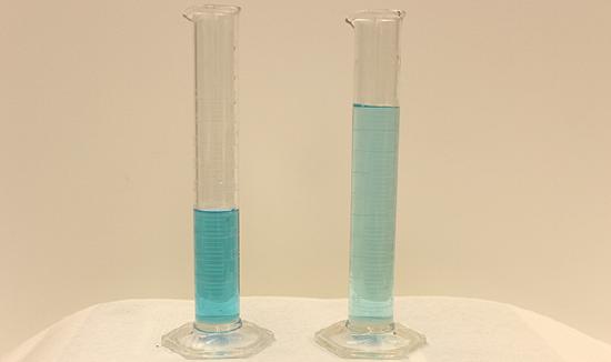
Dilution is the process whereby the concentration of a solution is lessened by the addition of solvent. For example, we might say that a glass of iced tea becomes increasingly diluted as the ice melts. The water from the melting ice increases the volume of the solvent (water) and the overall volume of the solution (iced tea), thereby reducing the relative concentrations of the solutes that give the beverage its taste (Figure \(\PageIndex{1}\)).

This figure shows two graduated cylinders side-by-side. The first has about half as much blue liquid as the second. The blue liquid is darker in the first cylinder than in the second. — Figure \(\PageIndex{1}\): Both solutions contain the same mass of copper nitrate. The solution on the right is more dilute because the copper nitrate is dissolved in more solvent. (credit: Mark Ott).

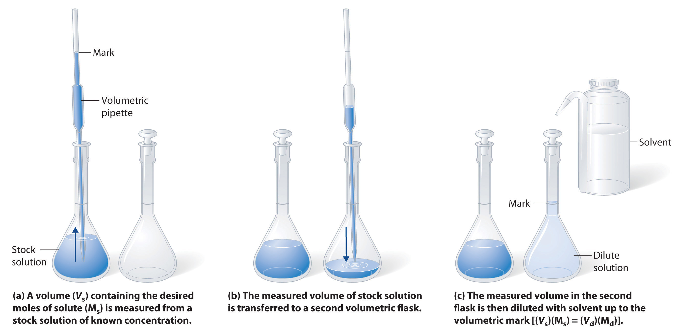
Dilution is also a common means of preparing solutions of a desired concentration. By adding solvent to a measured portion of a more concentrated stock solution, we can achieve a particular concentration. The procedure for preparing a solution of known concentration from a stock solution is shown in Figure \(\PageIndex{2}\). It requires calculating the number of moles of solute desired in the final volume of the more dilute solution and then calculating the volume of the stock solution that contains this amount of solute. Remember that diluting a given quantity of stock solution with solvent does not change the number of moles of solute present.

Figure \(\PageIndex{2}\): Preparation of a Solution of Known Concentration by Diluting a Stock Solution. (a) A volume (V_s) containing the desired moles of solute (M_s) is measured from a stock solution of known concentration. (b) The measured volume of stock solution is transferred to a second volumetric flask. (c) The measured volume in the second flask is then diluted with solvent up to the volumetric mark [(V_s)(M_s) = (V_d)(M_d)].

A simple mathematical relationship can be used to relate the volumes and concentrations of a solution before and after the dilution process. According to the definition of molarity, the molar amount of solute in a solution is equal to the product of the solution’s molarity and its volume in liters:

\[n=ML\]

Expressions like these may be written for a solution before and after it is diluted:

\[n_1=M_1L_1\]

\[n_2=M_2L_2\]

where the subscripts “1” and “2” refer to the solution before and after the dilution, respectively. Since the dilution process does not change the amount of solute in the solution,n₁ = n₂. Thus, these two equations may be set equal to one another:

\[M_1L_1=M_2L_2\]

This relation is commonly referred to as the dilution equation. Although we derived this equation using molarity as the unit of concentration and liters as the unit of volume, other units of concentration and volume may be used, so long as the units properly cancel per the factor-label method. Reflecting this versatility, the dilution equation is often written in the more general form:

\[C_1V_1=C_2V_2\]

where \(C\) and \(V\) are concentration and volume, respectively.

Example \(\PageIndex{1}\): Determining the Concentration of a Diluted Solution

If 0.850 L of a 5.00-M solution of copper nitrate, Cu(NO₃)₂, is diluted to a volume of 1.80 L by the addition of water, what is the molarity of the diluted solution?

Solution

We are given the volume and concentration of a stock solution, V₁ and C₁, and the volume of the resultant diluted solution, V₂. We need to find the concentration of the diluted solution, C₂. We thus rearrange the dilution equation in order to isolate C₂:

\[C_1V_1=C_2V_2 \nonumber\]

\[C_2=\dfrac{C_1V_1}{V_2} \nonumber\]

Since the stock solution is being diluted by more than two-fold (volume is increased from 0.85 L to 1.80 L), we would expect the diluted solution’s concentration to be less than one-half 5 M. We will compare this ballpark estimate to the calculated result to check for any gross errors in computation (for example, such as an improper substitution of the given quantities). Substituting the given values for the terms on the right side of this equation yields:

\[C_2=\mathrm{\dfrac{0.850\:L\times 5.00\:\dfrac{mol}{L}}{1.80\: L}}=2.36\:M \nonumber\]

This result compares well to our ballpark estimate (it’s a bit less than one-half the stock concentration, 5 M).

Exercise \(\PageIndex{1}\)

What is the concentration of the solution that results from diluting 25.0 mL of a 2.04-M solution of CH3OH to 500.0 mL?

Answer: 0.102 M \(CH_3OH\)

Example \(\PageIndex{2}\): Volume of a Diluted Solution

What volume of 0.12 M HBr can be prepared from 11 mL (0.011 L) of 0.45 M HBr?

Solution

We are given the volume and concentration of a stock solution, V₁ and C₁, and the concentration of the resultant diluted solution, C₂. We need to find the volume of the diluted solution, V₂. We thus rearrange the dilution equation in order to isolate V₂:

\[C_1V_1=C_2V_2 \nonumber\]

\[V_2=\dfrac{C_1V_1}{C_2} \nonumber\]

Since the diluted concentration (0.12 M) is slightly more than one-fourth the original concentration (0.45 M), we would expect the volume of the diluted solution to be roughly four times the original volume, or around 44 mL. Substituting the given values and solving for the unknown volume yields:

\[V_2=\dfrac{(0.45\:M)(0.011\: \ce L)}{(0.12\:M)} \nonumber\]

\[V_2=\mathrm{0.041\:L} \nonumber\]

The volume of the 0.12-M solution is 0.041 L (41 mL). The result is reasonable and compares well with our rough estimate.

Exercise \(\PageIndex{2}\)

A laboratory experiment calls for 0.125 M \(HNO_3\). What volume of 0.125 M \(HNO_3\) can be prepared from 0.250 L of 1.88 M \(HNO_3\)?

Answer: 3.76 L

Example \(\PageIndex{3}\): Volume of a Concentrated Solution Needed for Dilution

What volume of 1.59 M KOH is required to prepare 5.00 L of 0.100 M KOH?

Solution

We are given the concentration of a stock solution, C₁, and the volume and concentration of the resultant diluted solution, V₂ and C₂. We need to find the volume of the stock solution, V₁. We thus rearrange the dilution equation in order to isolate V₁:

\[C_1V_1=C_2V_2 \nonumber\]

\[V_1=\dfrac{C_2V_2}{C_1} \nonumber\]

Since the concentration of the diluted solution 0.100 M is roughly one-sixteenth that of the stock solution (1.59 M), we would expect the volume of the stock solution to be about one-sixteenth that of the diluted solution, or around 0.3 liters. Substituting the given values and solving for the unknown volume yields:

\[V_1=\dfrac{(0.100\:M)(5.00\:\ce L)}{1.59\:M} \nonumber\]

\[V_1=0.314\:\ce L \nonumber\]

Thus, we would need 0.314 L of the 1.59-M solution to prepare the desired solution. This result is consistent with our rough estimate.

Exercise \(\PageIndex{3}\)

What volume of a 0.575-M solution of glucose, C₆H₁₂O₆, can be prepared from 50.00 mL of a 3.00-M glucose solution?

Answer: 0.261 L

Summary

The dilution equation is a simple relation between concentrations and volumes of a solution before and after dilution.

Key Equations

\(M=\mathrm{\dfrac{mol\: solute}{L\: solution}}\)
C₁V₁ = C₂V₂

Glossary

dilution: process of adding solvent to a solution in order to lower the concentration of solutes

Contributors and Attributions

Paul Flowers (University of North Carolina - Pembroke), Klaus Theopold (University of Delaware) and Richard Langley (Stephen F. Austin State University) with contributing authors. Textbook content produced by OpenStax College is licensed under a Creative Commons Attribution License 4.0 license. Download for free at http://cnx.org/contents/85abf193-2bd...a7ac8df6@9.110).