3.7.2: Concentrations of Solutions

Last updated
Save as PDF

Page ID: 210734

$ \newcommand{\vecs}[1]{\overset { \scriptstyle \rightharpoonup} {\mathbf{#1}} } $ $ \newcommand{\vecd}[1]{\overset{-\!-\!\rightharpoonup}{\vphantom{a}\smash {#1}}} $$\newcommand{\id}{\mathrm{id}}$ $ \newcommand{\Span}{\mathrm{span}}$ $ \newcommand{\kernel}{\mathrm{null}\,}$ $ \newcommand{\range}{\mathrm{range}\,}$ $ \newcommand{\RealPart}{\mathrm{Re}}$ $ \newcommand{\ImaginaryPart}{\mathrm{Im}}$ $ \newcommand{\Argument}{\mathrm{Arg}}$ $ \newcommand{\norm}[1]{\| #1 \|}$ $ \newcommand{\inner}[2]{\langle #1, #2 \rangle}$ $ \newcommand{\Span}{\mathrm{span}}$ $\newcommand{\id}{\mathrm{id}}$ $ \newcommand{\Span}{\mathrm{span}}$ $ \newcommand{\kernel}{\mathrm{null}\,}$ $ \newcommand{\range}{\mathrm{range}\,}$ $ \newcommand{\RealPart}{\mathrm{Re}}$ $ \newcommand{\ImaginaryPart}{\mathrm{Im}}$ $ \newcommand{\Argument}{\mathrm{Arg}}$ $ \newcommand{\norm}[1]{\| #1 \|}$ $ \newcommand{\inner}[2]{\langle #1, #2 \rangle}$ $ \newcommand{\Span}{\mathrm{span}}$$\newcommand{\AA}{\unicode[.8,0]{x212B}}$

Learning Objectives

Define the concentration units of mass percentage, volume percentage, mass-volume percentage, parts-per-million (ppm), and parts-per-billion (ppb)
Perform computations relating a solution’s concentration and its components’ volumes and/or masses using these units\
Express concentrations of solution components using mole fraction and molality
Describe the effect of solute concentration on various solution properties (vapor pressure, boiling point, freezing point, and osmotic pressure)
Perform calculations using the mathematical equations that describe these various colligative effects

Last term, we introduced molarity, a very useful measurement unit for evaluating the concentration of solutions. However, molarity is only one measure of concentration. In this section, we will introduce some other units of concentration that are commonly used in various applications, either for convenience or by convention.

Mass Percentage

Last term, we also introduced percent composition as a measure of the relative amount of a given element in a compound. Percentages are also commonly used to express the composition of mixtures, including solutions. The mass percentage of a solution component is defined as the ratio of the component’s mass to the solution’s mass, expressed as a percentage:

\[ \text{mass percentage} = \dfrac{\text{mass of component}}{\text{mass of solution}} \times100\% \label{3.5.1}\]

We are generally most interested in the mass percentages of solutes, but it is also possible to compute the mass percentage of solvent.

Mass percentage is also referred to by similar names such as percent mass, percent weight, weight/weight percent, and other variations on this theme. The most common symbol for mass percentage is simply the percent sign, %, although more detailed symbols are often used including %mass, %weight, and (w/w)%. Use of these more detailed symbols can prevent confusion of mass percentages with other types of percentages, such as volume percentages (to be discussed later in this section).

Mass percentages are popular concentration units for consumer products. The label of a typical liquid bleach bottle (Figure $\PageIndex{1}$) cites the concentration of its active ingredient, sodium hypochlorite (NaOCl), as being 7.4%. A 100.0-g sample of bleach would therefore contain 7.4 g of NaOCl.

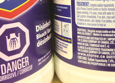
The sides of two cylindrical containers are shown. Each container’s label is partially visible. The left container’s label reads “Bleach.” The right label contains more information about the product including the phrase, “Contains: Sodium hypochlorite 7.4 %.”

Figure $\PageIndex{1}$: Liquid bleach is an aqueous solution of sodium hypochlorite (NaOCl). This brand has a concentration of 7.4% NaOCl by mass.

Example $\PageIndex{1}$: Calculation of Percent by Mass

A 5.0-g sample of spinal fluid contains 3.75 mg (0.00375 g) of glucose. What is the percent by mass of glucose in spinal fluid?

Solution

The spinal fluid sample contains roughly 4 mg of glucose in 5000 mg of fluid, so the mass fraction of glucose should be a bit less than one part in 1000, or about 0.1%. Substituting the given masses into the equation defining mass percentage yields:

\[\mathrm{\%\,glucose=\dfrac{3.75\;mg \;glucose \times \frac{1\;g}{1000\; mg}}{5.0\;g \;spinal\; fluid}=0.075\%}\]

The computed mass percentage agrees with our rough estimate (it’s a bit less than 0.1%).

Note that while any mass unit may be used to compute a mass percentage (mg, g, kg, oz, and so on), the same unit must be used for both the solute and the solution so that the mass units cancel, yielding a dimensionless ratio. In this case, we converted the units of solute in the numerator from mg to g to match the units in the denominator. We could just as easily have converted the denominator from g to mg instead. As long as identical mass units are used for both solute and solution, the computed mass percentage will be correct.

Exercise $\PageIndex{1}$

A bottle of a tile cleanser contains 135 g of HCl and 775 g of water. What is the percent by mass of HCl in this cleanser?

Answer: 14.8%

Example $\PageIndex{2}$: Calculations using Mass Percentage

“Concentrated” hydrochloric acid is an aqueous solution of 37.2% HCl that is commonly used as a laboratory reagent. The density of this solution is 1.19 g/mL. What mass of HCl is contained in 0.500 L of this solution?

Solution

The HCl concentration is near 40%, so a 100-g portion of this solution would contain about 40 g of HCl. Since the solution density isn’t greatly different from that of water (1 g/mL), a reasonable estimate of the HCl mass in 500 g (0.5 L) of the solution is about five times greater than that in a 100 g portion, or $\mathrm{5 \times 40 = 200\: g}$. To derive the mass of solute in a solution from its mass percentage, we need to know the corresponding mass of the solution. Using the solution density given, we can convert the solution’s volume to mass, and then use the given mass percentage to calculate the solute mass. This mathematical approach is outlined in this flowchart:

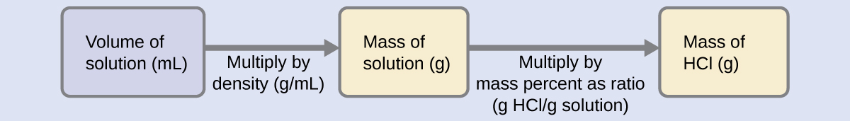
For proper unit cancellation, the 0.500-L volume is converted into 500 mL, and the mass percentage is expressed as a ratio, 37.2 g HCl/g solution:

\[ \mathrm{500\; mL\; solution \left(\dfrac{1.19\;g \;solution}{mL \;solution}\right) \left(\dfrac{37.2\;g\; HCl}{100\;g \;solution}\right)=221\;g\; HCl}\]

This mass of HCl is consistent with our rough estimate of approximately 200 g.

Exercise $\PageIndex{2}$

What volume of concentrated HCl solution contains 125 g of HCl?

Answer: 282 mL

Volume Percentage

Liquid volumes over a wide range of magnitudes are conveniently measured using common and relatively inexpensive laboratory equipment. The concentration of a solution formed by dissolving a liquid solute in a liquid solvent is therefore often expressed as a volume percentage, %vol or (v/v)%:

Example $\PageIndex{3}$: Calculations using Volume Percentage

Rubbing alcohol (isopropanol) is usually sold as a 70%vol aqueous solution. If the density of isopropyl alcohol is 0.785 g/mL, how many grams of isopropyl alcohol are present in a 355 mL bottle of rubbing alcohol?

Solution

Per the definition of volume percentage, the isopropanol volume is 70% of the total solution volume. Multiplying the isopropanol volume by its density yields the requested mass:

Exercise $\PageIndex{3}$

Wine is approximately 12% ethanol ($\ce{CH_3CH_2OH}$) by volume. Ethanol has a molar mass of 46.06 g/mol and a density 0.789 g/mL. How many moles of ethanol are present in a 750-mL bottle of wine?

Answer: 1.5 mol ethanol

Mass-Volume Percentage

“Mixed” percentage units, derived from the mass of solute and the volume of solution, are popular for certain biochemical and medical applications. A mass-volume percent is a ratio of a solute’s mass to the solution’s volume expressed as a percentage. The specific units used for solute mass and solution volume may vary, depending on the solution. For example, physiological saline solution, used to prepare intravenous fluids, has a concentration of 0.9% mass/volume (m/v), indicating that the composition is 0.9 g of solute per 100 mL of solution. The concentration of glucose in blood (commonly referred to as “blood sugar”) is also typically expressed in terms of a mass-volume ratio. Though not expressed explicitly as a percentage, its concentration is usually given in milligrams of glucose per deciliter (100 mL) of blood (Figure $\PageIndex{2}$).

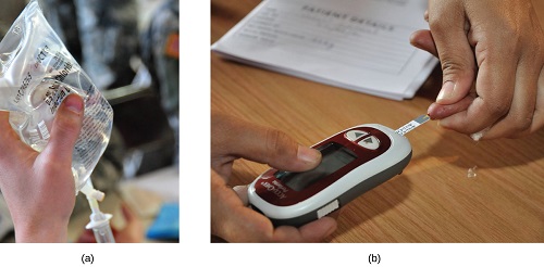
Two pictures are shown labeled a and b. Picture a depicts a clear, colorless solution in a plastic bag being held in a person’s hand. Picture b shows a person’s hand holding a detection meter with a digital readout screen while another hand holds someone’s finger up to the end of the meter. The meter is pressed to the drop of blood that is at the end of the person’s finger.

Figure $\PageIndex{2}$: “Mixed” mass-volume units are commonly encountered in medical settings. (a) The NaCl concentration of physiological saline is 0.9% (m/v). (b) This device measures glucose levels in a sample of blood. The normal range for glucose concentration in blood (fasting) is around 70–100 mg/dL. (credit a: modification of work by “The National Guard”/Flickr; credit b: modification of work by Biswarup Ganguly).

Parts per Million and Parts per Billion

Very low solute concentrations are often expressed using appropriately small units such as parts per million (ppm) or parts per billion (ppb). Like percentage (“part per hundred”) units, ppm and ppb may be defined in terms of masses, volumes, or mixed mass-volume units. There are also ppm and ppb units defined with respect to numbers of atoms and molecules.

The mass-based definitions of ppm and ppb are given here:

\[\text{ppm}=\dfrac{\text{mass solute}}{\text{mass solution}} \times 10^6\; \text{ppm} \label{3.5.3A}\]

\[\text{ppb}=\dfrac{\text{mass solute}}{\text{mass solution}} \times 10^9\; \text{ppb} \label{3.5.3B}\]

Both ppm and ppb are convenient units for reporting the concentrations of pollutants and other trace contaminants in water. Concentrations of these contaminants are typically very low in treated and natural waters, and their levels cannot exceed relatively low concentration thresholds without causing adverse effects on health and wildlife. For example, the EPA has identified the maximum safe level of fluoride ion in tap water to be 4 ppm. Inline water filters are designed to reduce the concentration of fluoride and several other trace-level contaminants in tap water (Figure $\PageIndex{3}$).

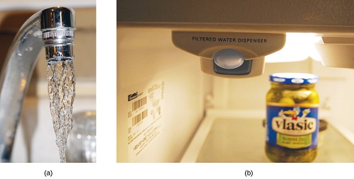
Figure $\PageIndex{3}$: (a) In some areas, trace-level concentrations of contaminants can render unfiltered tap water unsafe for drinking and cooking. (b) Inline water filters reduce the concentration of solutes in tap water. (credit a: modification of work by Jenn Durfey; credit b: modification of work by “vastateparkstaff”/Wikimedia commons).

Example $\PageIndex{4}$: Parts per Million and Parts per Billion Concentrations

According to the EPA, when the concentration of lead in tap water reaches 15 ppb, certain remedial actions must be taken. What is this concentration in ppm? At this concentration, what mass of lead (μg) would be contained in a typical glass of water (300 mL)?

Solution

The definitions of the ppm and ppb units may be used to convert the given concentration from ppb to ppm. Comparing these two unit definitions shows that ppm is 1000 times greater than ppb (1 ppm = 10³ ppb). Thus:

\[ \mathrm{15\; \cancel{ppb} \times \dfrac{1\; ppm}{10^3\;\cancel{ppb}} =0.015\; ppm}\]

The definition of the ppb unit may be used to calculate the requested mass if the mass of the solution is provided. However, only the volume of solution (300 mL) is given, so we must use the density to derive the corresponding mass. We can assume the density of tap water to be roughly the same as that of pure water (~1.00 g/mL), since the concentrations of any dissolved substances should not be very large. Rearranging the equation defining the ppb unit and substituting the given quantities yields:

\[\text{ppb}=\dfrac{\text{mass solute}}{\text{mass solution}} ×10^9\; \text{ppb}\]

\[\text{mass solute} = \dfrac{\text{ppb} \times \text{mass solution}}{10^9\;\text{ppb}}\]

\[\text{mass solute}=\mathrm{\dfrac{15\:ppb×300\:mL×\dfrac{1.00\:g}{mL}}{10^9\:ppb}=4.5 \times 10^{-6}\;g}\]

Finally, convert this mass to the requested unit of micrograms:

\[\mathrm{4.5 \times 10^{−6}\;g \times \dfrac{1\; \mu g}{10^{−6}\;g} =4.5\; \mu g}\]

Exercise $\PageIndex{4}$

A 50.0-g sample of industrial wastewater was determined to contain 0.48 mg of mercury. Express the mercury concentration of the wastewater in ppm and ppb units.

Answer: 9.6 ppm, 9600 ppb

The properties of a solution are different from those of either the pure solute(s) or solvent. Many solution properties are dependent upon the chemical identity of the solute. Compared to pure water, a solution of hydrogen chloride is more acidic, a solution of ammonia is more basic, a solution of sodium chloride is more dense, and a solution of sucrose is more viscous. There are a few solution properties, however, that depend only upon the total concentration of solute species, regardless of their identities. These colligative properties include vapor pressure lowering, boiling point elevation, freezing point depression, and osmotic pressure. This small set of properties is of central importance to many natural phenomena and technological applications, as will be described in this module.

Mole Fraction and Molality

Several units commonly used to express the concentrations of solution components were introduced in an earlier chapter of this text, each providing certain benefits for use in different applications. For example, molarity (M) is a convenient unit for use in stoichiometric calculations, since it is defined in terms of the molar amounts of solute species:

\[M=\dfrac{\text{mol solute}}{\text{L solution}} \label{11.5.1}\]

Because solution volumes vary with temperature, molar concentrations will likewise vary. When expressed as molarity, the concentration of a solution with identical numbers of solute and solvent species will be different at different temperatures, due to the contraction/expansion of the solution. More appropriate for calculations involving many colligative properties are mole-based concentration units whose values are not dependent on temperature. Two such units are mole fraction (introduced in the previous chapter on gases) and molality.

The mole fraction, $X$, of a component is the ratio of its molar amount to the total number of moles of all solution components:

\[X_\ce{A}=\dfrac{\text{mol A}}{\text{total mol of all components}} \label{11.5.2}\]

Molality is a concentration unit defined as the ratio of the numbers of moles of solute to the mass of the solvent in kilograms:

\[m=\dfrac{\text{mol solute}}{\text{kg solvent}} \label{11.5.3}\]

Since these units are computed using only masses and molar amounts, they do not vary with temperature and, thus, are better suited for applications requiring temperature-independent concentrations, including several colligative properties, as will be described in this chapter module.

Example $\PageIndex{5}$: Calculating Mole Fraction and Molality

The antifreeze in most automobile radiators is a mixture of equal volumes of ethylene glycol and water, with minor amounts of other additives that prevent corrosion. What are the (a) mole fraction and (b) molality of ethylene glycol, C_₂H_₄(OH)₂, in a solution prepared from $\mathrm{2.22 \times 10^3 \;g}$ of ethylene glycol and $\mathrm{2.00 \times 10^3\; g}$ of water (approximately 2 L of glycol and 2 L of water)?

Solution

(a) The mole fraction of ethylene glycol may be computed by first deriving molar amounts of both solution components and then substituting these amounts into the unit definition.

$\mathrm{mol\:C_2H_4(OH)_2=2220\:g×\dfrac{1\:mol\:C_2H_4(OH)_2}{62.07\:g\:C_2H_4(OH)_2}=35.8\:mol\:C_2H_4(OH)_2}$

$\mathrm{mol\:H_2O=2000\:g×\dfrac{1\:mol\:H_2O}{18.02\:g\:H_2O}=111\:mol\:H_2O}$

$X_\mathrm{ethylene\:glycol}=\mathrm{\dfrac{35.8\:mol\:C_2H_4(OH)_2}{(35.8+111)\:mol\: total}=0.245}$

Notice that mole fraction is a dimensionless property, being the ratio of properties with identical units (moles).

(b) To find molality, we need to know the moles of the solute and the mass of the solvent (in kg).

First, use the given mass of ethylene glycol and its molar mass to find the moles of solute:

\[\mathrm{2220\:g\:C_2H_4(OH)_2\left(\dfrac{mol\:C_2H_2(OH)_2}{62.07\:g}\right)=35.8\:mol\:C_2H_4(OH)_2}\]

Then, convert the mass of the water from grams to kilograms:

\[\mathrm{2000\: g\:H_2O\left(\dfrac{1\:kg}{1000\:g}\right)=2\: kg\:H_2O}\]

Finally, calculate molarity per its definition:

$\begin{align}
\ce{molality}&=\mathrm{\dfrac{mol\: solute}{kg\: solvent}}\\
\ce{molality}&=\mathrm{\dfrac{35.8\:mol\:C_2H_4(OH)_2}{2\:kg\:H_2O}}\\
\ce{molality}&=17.9\:m
\end{align}$

Exercise $\PageIndex{5}$

What are the mole fraction and molality of a solution that contains 0.850 g of ammonia, NH₃, dissolved in 125 g of water?

Answer: 7.14 × 10⁻³; 0.399 m

Example $\PageIndex{6}$: Converting Mole Fraction and Molal Concentrations

Calculate the mole fraction of solute and solvent in a 3.0 m solution of sodium chloride.

Solution

Converting from one concentration unit to another is accomplished by first comparing the two unit definitions. In this case, both units have the same numerator (moles of solute) but different denominators. The provided molal concentration may be written as:

\[\mathrm{\dfrac{3.0\;mol\; NaCl}{1.0\; kg\; H_2O}} \label{11.5.X}\]

The numerator for this solution’s mole fraction is, therefore, 3.0 mol NaCl. The denominator may be computed by deriving the molar amount of water corresponding to 1.0 kg

$\mathrm{1.0\:kg\:H_2O\left(\dfrac{1000\:g}{1\:kg}\right)\left(\dfrac{mol\:H_2O}{18.02\:g}\right)=55\:mol\:H_2O}$

and then substituting these molar amounts into the definition for mole fraction.

\[\begin{align*}
X_\mathrm{H_2O}&=\mathrm{\dfrac{mol\:H_2O}{mol\: NaCl + mol\:H_2O}}\\
X_\mathrm{H_2O}&=\mathrm{\dfrac{55\:mol\:H_2O}{3.0\:mol\: NaCl+55\:mol\:H_2O}}\\
X_\mathrm{H_2O}&=0.95\\
X_\mathrm{NaCl}&=\mathrm{\dfrac{mol\: NaCl}{mol\: NaCl+mol\:H_2O}}\\
X_\mathrm{NaCl}&=\mathrm{\dfrac{3.0\:mol\:NaCl}{3.0\:mol\: NaCl+55\:mol\:H_2O}}\\
X_\mathrm{NaCl}&=0.052
\end{align*}\]

Exercise $\PageIndex{6}$

The mole fraction of iodine, $\mathrm{I_2}$, dissolved in dichloromethane, $\mathrm{CH_2Cl_2}$, is 0.115. What is the molal concentration, m, of iodine in this solution?

Answer: 1.50 m

Vapor Pressure Lowering

As described in the previous unit, the equilibrium vapor pressure of a liquid is the pressure exerted by its gaseous phase when vaporization and condensation are occurring at equal rates:

\[ \text{liquid} \rightleftharpoons \text{gas} \label{11.5.4}\]

Dissolving a nonvolatile substance in a volatile liquid results in a lowering of the liquid’s vapor pressure. This phenomenon can be rationalized by considering the effect of added solute molecules on the liquid's vaporization and condensation processes. To vaporize, solvent molecules must be present at the surface of the solution. The presence of solute decreases the surface area available to solvent molecules and thereby reduces the rate of solvent vaporization. Since the rate of condensation is unaffected by the presence of solute, the net result is that the vaporization-condensation equilibrium is achieved with fewer solvent molecules in the vapor phase (i.e., at a lower vapor pressure) (Figure $\PageIndex{4}$). While this kinetic interpretation is useful, it does not account for several important aspects of the colligative nature of vapor pressure lowering. A more rigorous explanation involves the property of entropy, a topic of discussion in a later text chapter on thermodynamics. For purposes of understanding the lowering of a liquid's vapor pressure, it is adequate to note that the greater entropy of a solution in comparison to its separate solvent and solute serves to effectively stabilize the solvent molecules and hinder their vaporization. A lower vapor pressure results, and a correspondingly higher boiling point as described in the next section of this module.

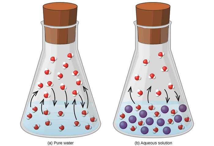
Figure $\PageIndex{4}$: The presence of nonvolatile solutes lowers the vapor pressure of a solution by impeding the evaporation of solvent molecules.

The relationship between the vapor pressures of solution components and the concentrations of those components is described by Raoult’s law: The partial pressure exerted by any component of an ideal solution is equal to the vapor pressure of the pure component multiplied by its mole fraction in the solution.

\[P_\ce{A}=X_\ce{A}P^\circ_\ce{A} \label{11.5.5}\]

where P_A is the partial pressure exerted by component A in the solution, $P^\circ_\ce{A}$ is the vapor pressure of pure A, and X_A is the mole fraction of A in the solution. (Mole fraction is a concentration unit introduced in the chapter on gases.)

Elevation of the Boiling Point of a Solvent

As described in the chapter on liquids and solids, the boiling point of a liquid is the temperature at which its vapor pressure is equal to ambient atmospheric pressure. Since the vapor pressure of a solution is lowered due to the presence of nonvolatile solutes, it stands to reason that the solution’s boiling point will subsequently be increased. Compared to pure solvent, a solution, therefore, will require a higher temperature to achieve any given vapor pressure, including one equivalent to that of the surrounding atmosphere. The increase in boiling point observed when nonvolatile solute is dissolved in a solvent, $ΔT_b$, is called boiling point elevation and is directly proportional to the molal concentration of solute species:

\[ΔT_b=K_bm \label{11.5.8}\]

where

$K_\ce{b}$ is the boiling point elevation constant, or the ebullioscopic constant and
$m$ is the molal concentration (molality) of all solute species.

Boiling point elevation constants are characteristic properties that depend on the identity of the solvent. Values of K_b for several solvents are listed in Table $\PageIndex{1}$.

Table $\PageIndex{1}$: Boiling Point Elevation and Freezing Point Depression Constants for Several Solvents
Solvent	Boiling Point (°C at 1 atm)	Kb (Cm⁻¹)	Freezing Point (°C at 1 atm)	Kf (Cm−1)
water	100.0	0.512	0.0	1.86
hydrogen acetate	118.1	3.07	16.6	3.9
benzene	80.1	2.53	5.5	5.12
chloroform	61.26	3.63	−63.5	4.68
nitrobenzene	210.9	5.24	5.67	8.1

The extent to which the vapor pressure of a solvent is lowered and the boiling point is elevated depends on the total number of solute particles present in a given amount of solvent, not on the mass or size or chemical identities of the particles. A 1 m aqueous solution of sucrose (342 g/mol) and a 1 m aqueous solution of ethylene glycol (62 g/mol) will exhibit the same boiling point because each solution has one mole of solute particles (molecules) per kilogram of solvent.

Example $\PageIndex{7}$: Calculating the Boiling Point of a Solution

What is the boiling point of a 0.33 m solution of a nonvolatile solute in benzene?

Solution

Use the equation relating boiling point elevation to solute molality to solve this problem in two steps.

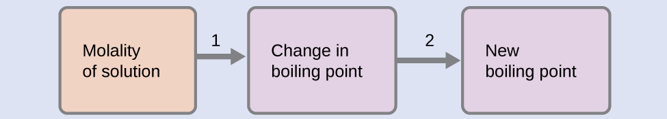
Calculate the change in boiling point.

$ΔT_\ce{b}=K_\ce{b}m=2.53\:°\ce C\:m^{−1}×0.33\:m=0.83\:°\ce C$

Add the boiling point elevation to the pure solvent’s boiling point.
$\mathrm{Boiling\: temperature=80.1\:°C+0.83\:°C=80.9\:°C}$

Exercise $\PageIndex{7}$

What is the boiling point of the antifreeze described in Example $\PageIndex{4}$?

Answer: 109.2 °C

Example $\PageIndex{8}$: The Boiling Point of an Iodine Solution

Find the boiling point of a solution of 92.1 g of iodine, I₂, in 800.0 g of chloroform, CHCl₃, assuming that the iodine is nonvolatile and that the solution is ideal.

Solution

We can solve this problem using four steps.

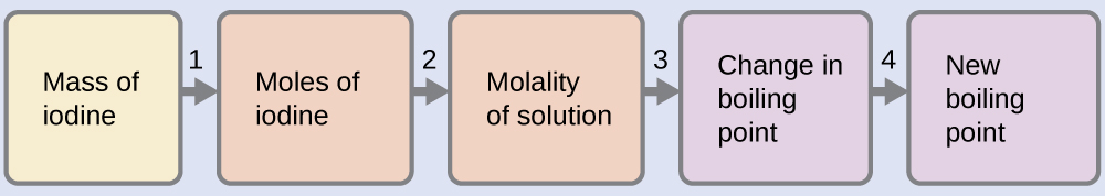
This is a diagram with three boxes connected with two arrows pointing to the right. The first box is labeled, “Molality of solution,” followed by an arrow labeled, “1,” pointing to a second box labeled, “Change in boiling point,” followed by an arrow labeled, “2,” pointing to a third box labeled, “New boiling point.”

Convert from grams to moles of I₂ using the molar mass of I₂ in the unit conversion factor.
Result: 0.363 mol
Determine the molality of the solution from the number of moles of solute and the mass of solvent, in kilograms.
Result: 0.454 m
Use the direct proportionality between the change in boiling point and molal concentration to determine how much the boiling point changes.
Result: 1.65 °C
Determine the new boiling point from the boiling point of the pure solvent and the change.
Result: 62.91 °C

Check each result as a self-assessment.

Exercise $\PageIndex{8}$

What is the boiling point of a solution of 1.0 g of glycerin, C₃H₅(OH)₃, in 47.8 g of water? Assume an ideal solution.

Answer: 100.12 °C

Distillation of Solutions

Distillation is a technique for separating the components of mixtures that is widely applied in both in the laboratory and in industrial settings. It is used to refine petroleum, to isolate fermentation products, and to purify water. This separation technique involves the controlled heating of a sample mixture to selectively vaporize, condense, and collect one or more components of interest. A typical apparatus for laboratory-scale distillations is shown in Figure $\PageIndex{5}$.

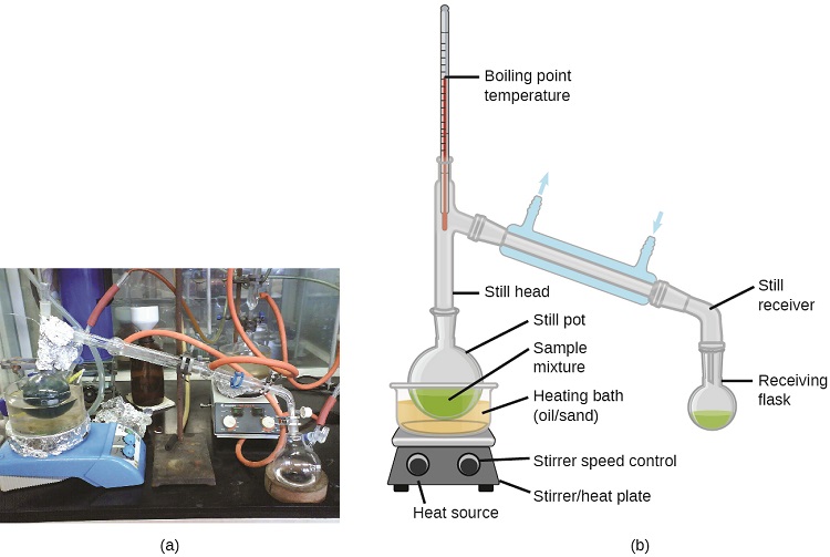
Figure $\PageIndex{5}$: A typical laboratory distillation unit is shown in (a) a photograph and (b) a schematic diagram of the components. (credit a: modification of work by “Rifleman82”/Wikimedia commons; credit b: modification of work by “Slashme”/Wikimedia Commons)

Oil refineries use large-scale fractional distillation to separate the components of crude oil. The crude oil is heated to high temperatures at the base of a tall fractionating column, vaporizing many of the components that rise within the column. As vaporized components reach adequately cool zones during their ascent, they condense and are collected. The collected liquids are simpler mixtures of hydrocarbons and other petroleum compounds that are of appropriate composition for various applications (e.g., diesel fuel, kerosene, gasoline), as depicted in Figure $\PageIndex{6}$.

$This figure contains a photo of a refinery, showing large columnar structures. A diagram of a fractional distillation column used in separating crude oil is also shown. Near the bottom of the column, an arrow pointing into the column shows a point of entry for heated crude oil. The column contains several layers at which different components are removed. At the very bottom, residue materials are removed as indicated by an arrow out of the column. At each successive level, different materials are removed proceeding from the bottom to the top of the column. The materials are fuel oil, followed by diesel oil, kerosene, naptha, gasoline, and refinery gas at the very top. To the right of the column diagram, a double sided arrow is shown that is blue at the top and gradually changes color to red moving downward. The blue top of the arrow is labeled, “small molecules: low boiling point, very volatile, flows easily, ignites easily.” The red bottom of the arrow is labeled, “large molecules: high boiling point, not very volatile, does not flow easily, does not ignite easily.”$

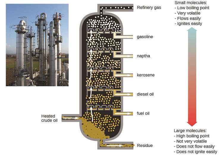
Figure $\PageIndex{6}$: Crude oil is a complex mixture that is separated by large-scale fractional distillation to isolate various simpler mixtures.

Depression of the Freezing Point of a Solvent

Solutions freeze at lower temperatures than pure liquids. This phenomenon is exploited in “de-icing” schemes that use salt (Figure $\PageIndex{7}$), calcium chloride, or urea to melt ice on roads and sidewalks, and in the use of ethylene glycol as an “antifreeze” in automobile radiators. Seawater freezes at a lower temperature than fresh water, and so the Arctic and Antarctic oceans remain unfrozen even at temperatures below 0 °C (as do the body fluids of fish and other cold-blooded sea animals that live in these oceans).

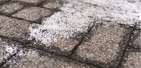
This is a photo of damp brick pavement on which a white crystalline material has been spread.

Figure $\PageIndex{7}$: Rock salt (NaCl), calcium chloride (CaCl₂), or a mixture of the two are used to melt ice. (credit: modification of work by Eddie Welker)

The decrease in freezing point of a dilute solution compared to that of the pure solvent, ΔT_f, is called the freezing point depression and is directly proportional to the molal concentration of the solute

\[ΔT_\ce{f}=K_\ce{f}m \label{11.5.9}\]

where

$m$ is the molal concentration of the solute in the solvent and
$K_f$ is called the freezing point depression constant (or cryoscopic constant).

Just as for boiling point elevation constants, these are characteristic properties whose values depend on the chemical identity of the solvent. Values of K_f for several solvents are listed in Table $\PageIndex{1}$.

Example $\PageIndex{9}$: Calculation of the Freezing Point of a Solution

What is the freezing point of the 0.33 m solution of a nonvolatile nonelectrolyte solute in benzene described in Example $\PageIndex{4}$?

Solution

Use the equation relating freezing point depression to solute molality to solve this problem in two steps.

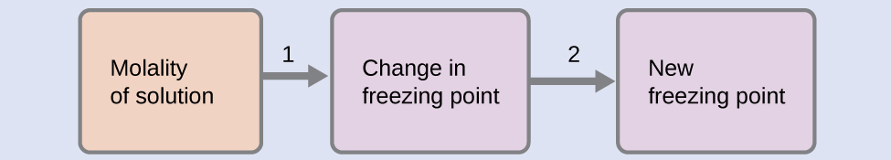
This is a diagram with three boxes connected with two arrows pointing to the right. The first box is labeled, “Molality of solution,” followed by an arrow labeled, “1,” pointing to a second box labeled, “Change in freezing point,” followed by an arrow labeled, “2” pointing to a third box labeled, “New freezing point.”

Calculate the change in freezing point. \[ΔT_\ce{f}=K_\ce{f}m=5.12\:°\ce C\:m^{−1}×0.33\:m=1.7\:°\ce C\]
Subtract the freezing point change observed from the pure solvent’s freezing point. [\mathrm{Freezing\: Temperature=5.5\:°C−1.7\:°C=3.8\:°C}\]

Exercise $\PageIndex{9}$

What is the freezing point of a 1.85 m solution of a nonvolatile nonelectrolyte solute in nitrobenzene?

Answer: −9.3 °C

Colligative Properties and De-Icing

Sodium chloride and its group 2 analogs calcium and magnesium chloride are often used to de-ice roadways and sidewalks, due to the fact that a solution of any one of these salts will have a freezing point lower than 0 °C, the freezing point of pure water. The group 2 metal salts are frequently mixed with the cheaper and more readily available sodium chloride (“rock salt”) for use on roads, since they tend to be somewhat less corrosive than the NaCl, and they provide a larger depression of the freezing point, since they dissociate to yield three particles per formula unit, rather than two particles like the sodium chloride.

Because these ionic compounds tend to hasten the corrosion of metal, they would not be a wise choice to use in antifreeze for the radiator in your car or to de-ice a plane prior to takeoff. For these applications, covalent compounds, such as ethylene or propylene glycol, are often used. The glycols used in radiator fluid not only lower the freezing point of the liquid, but they elevate the boiling point, making the fluid useful in both winter and summer. Heated glycols are often sprayed onto the surface of airplanes prior to takeoff in inclement weather in the winter to remove ice that has already formed and prevent the formation of more ice, which would be particularly dangerous if formed on the control surfaces of the aircraft (Video $\PageIndex{1}$).

Video $\PageIndex{1}$: Freezing point depression is exploited to remove ice from the control surfaces of aircraft.

Phase Diagram for an Aqueous Solution of a Nonelectrolyte

The colligative effects on vapor pressure, boiling point, and freezing point described in the previous section are conveniently summarized by comparing the phase diagrams for a pure liquid and a solution derived from that liquid. Phase diagrams for water and an aqueous solution are shown in Figure $\PageIndex{8}$.

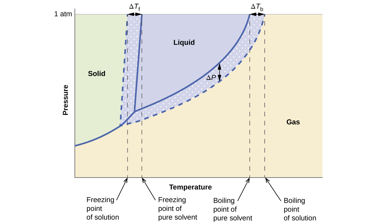
Figure $\PageIndex{8}$: These phase diagrams show water (solid curves) and an aqueous solution of nonelectrolyte (dashed curves).

The liquid-vapor curve for the solution is located beneath the corresponding curve for the solvent, depicting the vapor pressure lowering, ΔP, that results from the dissolution of nonvolatile solute. Consequently, at any given pressure, the solution’s boiling point is observed at a higher temperature than that for the pure solvent, reflecting the boiling point elevation, ΔT_b, associated with the presence of nonvolatile solute. The solid-liquid curve for the solution is displaced left of that for the pure solvent, representing the freezing point depression, ΔTf, that accompanies solution formation. Finally, notice that the solid-gas curves for the solvent and its solution are identical. This is the case for many solutions comprising liquid solvents and nonvolatile solutes. Just as for vaporization, when a solution of this sort is frozen, it is actually just the solvent molecules that undergo the liquid-to-solid transition, forming pure solid solvent that excludes solute species. The solid and gaseous phases, therefore, are composed solvent only, and so transitions between these phases are not subject to colligative effects.

Determination of Molar Masses

Changes in freezing point, boiling point, and vapor pressure are directly proportional to the concentration of solute present. Consequently, we can use a measurement of one of these properties to determine the molar mass of the solute from the measurements.

Example $\PageIndex{10}$: Determining Molar Mass from Freezing Point Depression

A solution of 4.00 g of a nonelectrolyte dissolved in 55.0 g of benzene is found to freeze at 2.32 °C. What is the molar mass of this compound?

Solution

We can solve this problem using the following steps.

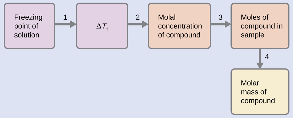
Determine the change in freezing point from the observed freezing point and the freezing point of pure benzene (Table 11.5.1).
$ΔT_\ce{f}=\mathrm{5.5\:°C−2.32\:°C=3.2\:°C}$
Determine the molal concentration from K_f, the freezing point depression constant for benzene (Table 11.5.1), and ΔT_f.
$ΔT_\ce{f}=K_\ce{f}m$
$m=\dfrac{ΔT_\ce{f}}{K_\ce{f}}=\dfrac{3.2\:°\ce C}{5.12\:°\ce C m^{−1}}=0.63\:m$
Determine the number of moles of compound in the solution from the molal concentration and the mass of solvent used to make the solution.
$\mathrm{Moles\: of\: solute=\dfrac{0.62\:mol\: solute}{1.00\cancel{kg\: solvent}}×0.0550\cancel{kg\: solvent}=0.035\:mol}$
Determine the molar mass from the mass of the solute and the number of moles in that mass.
$\mathrm{Molar\: mass=\dfrac{4.00\:g}{0.034\:mol}=1.2×10^2\:g/mol}$

Exercise $\PageIndex{10}$

A solution of 35.7 g of a nonelectrolyte in 220.0 g of chloroform has a boiling point of 64.5 °C. What is the molar mass of this compound?

Answer: 1.8 × 10² g/mol

Example $\PageIndex{11}$: Determination of a Molar Mass from Osmotic Pressure

A 0.500 L sample of an aqueous solution containing 10.0 g of hemoglobin has an osmotic pressure of 5.9 torr at 22 °C. What is the molar mass of hemoglobin?

Solution

Here is one set of steps that can be used to solve the problem:

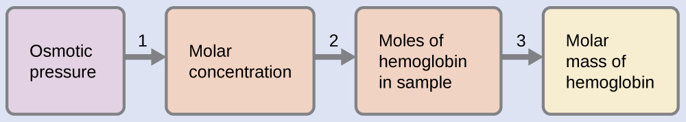
Convert the osmotic pressure to atmospheres, then determine the molar concentration from the osmotic pressure.
\[\Pi=\mathrm{\dfrac{5.9\:torr×1\:atm}{760\:torr}=7.8×10^{−3}\:atm}\]
\[\Pi=MRT\]
$M=\dfrac{Π}{RT}=\mathrm{\dfrac{7.8×10^{−3}\:atm}{(0.08206\:L\: atm/mol\: K)(295\:K)}=3.2×10^{−4}\:M}$
Determine the number of moles of hemoglobin in the solution from the concentration and the volume of the solution.
$\mathrm{moles\: of\: hemoglobin=\dfrac{3.2×10^{−4}\:mol}{1\cancel{L\: solution}}×0.500\cancel{L\: solution}=1.6×10^{−4}\:mol}$
Determine the molar mass from the mass of hemoglobin and the number of moles in that mass.
$\mathrm{molar\: mass=\dfrac{10.0\:g}{1.6×10^{−4}\:mol}=6.2×10^4\:g/mol}$

Exercise $\PageIndex{11}$

What is the molar mass of a protein if a solution of 0.02 g of the protein in 25.0 mL of solution has an osmotic pressure of 0.56 torr at 25 °C?

Answer: 2.7 × 10⁴ g/mol

Colligative Properties of Electrolytes

As noted previously in this module, the colligative properties of a solution depend only on the number, not on the kind, of solute species dissolved. For example, 1 mole of any nonelectrolyte dissolved in 1 kilogram of solvent produces the same lowering of the freezing point as does 1 mole of any other nonelectrolyte. However, 1 mole of sodium chloride (an electrolyte) forms 2 moles of ions when dissolved in solution. Each individual ion produces the same effect on the freezing point as a single molecule does.

Example $\PageIndex{13}$: The Freezing Point of a Solution of an Electrolyte

The concentration of ions in seawater is approximately the same as that in a solution containing 4.2 g of NaCl dissolved in 125 g of water. Assume that each of the ions in the NaCl solution has the same effect on the freezing point of water as a nonelectrolyte molecule, and determine the freezing temperature the solution (which is approximately equal to the freezing temperature of seawater).

Solution

We can solve this problem using the following series of steps.

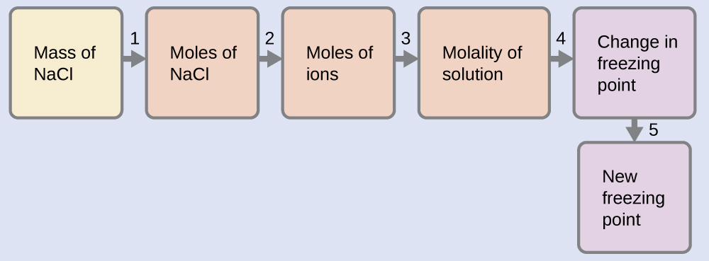
Convert from grams to moles of NaCl using the molar mass of NaCl in the unit conversion factor. Result: 0.072 mol NaCl
Determine the number of moles of ions present in the solution using the number of moles of ions in 1 mole of NaCl as the conversion factor (2 mol ions/1 mol NaCl). Result: 0.14 mol ions
Determine the molality of the ions in the solution from the number of moles of ions and the mass of solvent, in kilograms. Result: 1.1 m
Use the direct proportionality between the change in freezing point and molal concentration to determine how much the freezing point changes. Result: 2.0 °C
Determine the new freezing point from the freezing point of the pure solvent and the change. Result: −2.0 °C

Check each result as a self-assessment.

Exercise $\PageIndex{13}$

Assume that each of the ions in calcium chloride, CaCl₂, has the same effect on the freezing point of water as a nonelectrolyte molecule. Calculate the freezing point of a solution of 0.724 g of CaCl₂ in 175 g of water.

Answer: −0.208 °C

Assuming complete dissociation, a 1.0 m aqueous solution of NaCl contains 2.0 mole of ions (1.0 mol Na⁺ and 1.0 mol Cl⁻) per each kilogram of water, and its freezing point depression is expected to be

\[ΔT_\ce{f}=\mathrm{2.0\:mol\: ions/kg\: water×1.86\:°C\: kg\: water/mol\: ion=3.7\:°C.} \label{11.5.11}\]

When this solution is actually prepared and its freezing point depression measured, however, a value of 3.4 °C is obtained. Similar discrepancies are observed for other ionic compounds, and the differences between the measured and expected colligative property values typically become more significant as solute concentrations increase. These observations suggest that the ions of sodium chloride (and other strong electrolytes) are not completely dissociated in solution.

To account for this and avoid the errors accompanying the assumption of total dissociation, an experimentally measured parameter named in honor of Nobel Prize-winning German chemist Jacobus Henricus van’t Hoff is used. The van’t Hoff factor (i) is defined as the ratio of solute particles in solution to the number of formula units dissolved:

\[i=\dfrac{\textrm{moles of particles in solution}}{\textrm{moles of formula units dissolved}} \label{11.5.12}\]

Values for measured van’t Hoff factors for several solutes, along with predicted values assuming complete dissociation, are shown in Table $\PageIndex{2}$.

Table $\PageIndex{2}$: Expected and Observed van’t Hoff Factors for Several 0.050 m Aqueous Electrolyte Solutions
Electrolyte	Particles in Solution	i (Predicted)	i (Measured)
HCl	H⁺, Cl⁻	2	1.9
NaCl	Na⁺, Cl⁻	2	1.9
MgSO₄	Mg²⁺, $\ce{SO4^2-}$	2	1.3
MgCl₂	Mg²⁺, 2Cl⁻	3	2.7
FeCl₃	Fe³⁺, 3Cl⁻	4	3.4
glucose (a non-electrolyte)	C₁₂H₂₂O₁₁	1	1.0

In 1923, the chemists Peter Debye and Erich Hückel proposed a theory to explain the apparent incomplete ionization of strong electrolytes. They suggested that although interionic attraction in an aqueous solution is very greatly reduced by solvation of the ions and the insulating action of the polar solvent, it is not completely nullified. The residual attractions prevent the ions from behaving as totally independent particles (Figure $\PageIndex{9}$). In some cases, a positive and negative ion may actually touch, giving a solvated unit called an ion pair. Thus, the activity, or the effective concentration, of any particular kind of ion is less than that indicated by the actual concentration. Ions become more and more widely separated the more dilute the solution, and the residual interionic attractions become less and less. Thus, in extremely dilute solutions, the effective concentrations of the ions (their activities) are essentially equal to the actual concentrations. Note that the van’t Hoff factors for the electrolytes in Table $\PageIndex{2}$ are for 0.05 m solutions, at which concentration the value of i for NaCl is 1.9, as opposed to an ideal value of 2.

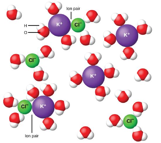
Figure $\PageIndex{9}$: Ions become more and more widely separated the more dilute the solution, and the residual interionic attractions become less.

Summary

Video $\PageIndex{2}$: An overview of concentration units for solutions.

In addition to molarity, a number of other solution concentration units are used in various applications. Percentage concentrations based on the solution components’ masses, volumes, or both are useful for expressing relatively high concentrations, whereas lower concentrations are conveniently expressed using ppm or ppb units. These units are popular in environmental, medical, and other fields where mole-based units such as molarity are not as commonly used.

Properties of a solution that depend only on the concentration of solute particles are called colligative properties. They include changes in the vapor pressure, boiling point, and freezing point of the solvent in the solution. The magnitudes of these properties depend only on the total concentration of solute particles in solution, not on the type of particles. Ionic compounds may not completely dissociate in solution due to activity effects, in which case observed colligative effects may be less than predicted.

Key Equations

ΔT_b = K_bm
ΔT_f = K_fm
Π = MRT

Footnotes

A nonelectrolyte shown for comparison.

Glossary

mass percentage: ratio of solute-to-solution mass expressed as a percentage

mass-volume percent: ratio of solute mass to solution volume, expressed as a percentage

parts per billion (ppb): ratio of solute-to-solution mass multiplied by 10⁹

parts per million (ppm): ratio of solute-to-solution mass multiplied by 10⁶

volume percentage: ratio of solute-to-solution volume expressed as a percentage

boiling point elevation: elevation of the boiling point of a liquid by addition of a solute

boiling point elevation constant: the proportionality constant in the equation relating boiling point elevation to solute molality; also known as the ebullioscopic constant

colligative property: property of a solution that depends only on the concentration of a solute species

freezing point depression: lowering of the freezing point of a liquid by addition of a solute

freezing point depression constant: (also, cryoscopic constant) proportionality constant in the equation relating freezing point depression to solute molality

ion pair: solvated anion/cation pair held together by moderate electrostatic attraction

molality (m): a concentration unit defined as the ratio of the numbers of moles of solute to the mass of the solvent in kilograms

van’t Hoff factor (i): the ratio of the number of moles of particles in a solution to the number of moles of formula units dissolved in the solution

Contributors and Attributions

Paul Flowers (University of North Carolina - Pembroke), Klaus Theopold (University of Delaware) and Richard Langley (Stephen F. Austin State University) with contributing authors. Textbook content produced by OpenStax College is licensed under a Creative Commons Attribution License 4.0 license. Download for free at http://cnx.org/contents/85abf193-2bd...a7ac8df6@9.110).
Adelaide Clark, Oregon Institute of Technology
Crash Course Chemistry: Crash Course is a division of Complexly and videos are free to stream for educational purposes.

Feedback

Have feedback to give about this text? Click here.

Found a typo and want extra credit? Click here.