
3.0.1: Atomic Spectroscopy and the deBroglie Wavelength
- Page ID
- 210681
\( \newcommand{\vecs}[1]{\overset { \scriptstyle \rightharpoonup} {\mathbf{#1}} } \)
\( \newcommand{\vecd}[1]{\overset{-\!-\!\rightharpoonup}{\vphantom{a}\smash {#1}}} \)
\( \newcommand{\id}{\mathrm{id}}\) \( \newcommand{\Span}{\mathrm{span}}\)
( \newcommand{\kernel}{\mathrm{null}\,}\) \( \newcommand{\range}{\mathrm{range}\,}\)
\( \newcommand{\RealPart}{\mathrm{Re}}\) \( \newcommand{\ImaginaryPart}{\mathrm{Im}}\)
\( \newcommand{\Argument}{\mathrm{Arg}}\) \( \newcommand{\norm}[1]{\| #1 \|}\)
\( \newcommand{\inner}[2]{\langle #1, #2 \rangle}\)
\( \newcommand{\Span}{\mathrm{span}}\)
\( \newcommand{\id}{\mathrm{id}}\)
\( \newcommand{\Span}{\mathrm{span}}\)
\( \newcommand{\kernel}{\mathrm{null}\,}\)
\( \newcommand{\range}{\mathrm{range}\,}\)
\( \newcommand{\RealPart}{\mathrm{Re}}\)
\( \newcommand{\ImaginaryPart}{\mathrm{Im}}\)
\( \newcommand{\Argument}{\mathrm{Arg}}\)
\( \newcommand{\norm}[1]{\| #1 \|}\)
\( \newcommand{\inner}[2]{\langle #1, #2 \rangle}\)
\( \newcommand{\Span}{\mathrm{span}}\) \( \newcommand{\AA}{\unicode[.8,0]{x212B}}\)
\( \newcommand{\vectorA}[1]{\vec{#1}} % arrow\)
\( \newcommand{\vectorAt}[1]{\vec{\text{#1}}} % arrow\)
\( \newcommand{\vectorB}[1]{\overset { \scriptstyle \rightharpoonup} {\mathbf{#1}} } \)
\( \newcommand{\vectorC}[1]{\textbf{#1}} \)
\( \newcommand{\vectorD}[1]{\overrightarrow{#1}} \)
\( \newcommand{\vectorDt}[1]{\overrightarrow{\text{#1}}} \)
\( \newcommand{\vectE}[1]{\overset{-\!-\!\rightharpoonup}{\vphantom{a}\smash{\mathbf {#1}}}} \)
\( \newcommand{\vecs}[1]{\overset { \scriptstyle \rightharpoonup} {\mathbf{#1}} } \)
\( \newcommand{\vecd}[1]{\overset{-\!-\!\rightharpoonup}{\vphantom{a}\smash {#1}}} \)
\(\newcommand{\avec}{\mathbf a}\) \(\newcommand{\bvec}{\mathbf b}\) \(\newcommand{\cvec}{\mathbf c}\) \(\newcommand{\dvec}{\mathbf d}\) \(\newcommand{\dtil}{\widetilde{\mathbf d}}\) \(\newcommand{\evec}{\mathbf e}\) \(\newcommand{\fvec}{\mathbf f}\) \(\newcommand{\nvec}{\mathbf n}\) \(\newcommand{\pvec}{\mathbf p}\) \(\newcommand{\qvec}{\mathbf q}\) \(\newcommand{\svec}{\mathbf s}\) \(\newcommand{\tvec}{\mathbf t}\) \(\newcommand{\uvec}{\mathbf u}\) \(\newcommand{\vvec}{\mathbf v}\) \(\newcommand{\wvec}{\mathbf w}\) \(\newcommand{\xvec}{\mathbf x}\) \(\newcommand{\yvec}{\mathbf y}\) \(\newcommand{\zvec}{\mathbf z}\) \(\newcommand{\rvec}{\mathbf r}\) \(\newcommand{\mvec}{\mathbf m}\) \(\newcommand{\zerovec}{\mathbf 0}\) \(\newcommand{\onevec}{\mathbf 1}\) \(\newcommand{\real}{\mathbb R}\) \(\newcommand{\twovec}[2]{\left[\begin{array}{r}#1 \\ #2 \end{array}\right]}\) \(\newcommand{\ctwovec}[2]{\left[\begin{array}{c}#1 \\ #2 \end{array}\right]}\) \(\newcommand{\threevec}[3]{\left[\begin{array}{r}#1 \\ #2 \\ #3 \end{array}\right]}\) \(\newcommand{\cthreevec}[3]{\left[\begin{array}{c}#1 \\ #2 \\ #3 \end{array}\right]}\) \(\newcommand{\fourvec}[4]{\left[\begin{array}{r}#1 \\ #2 \\ #3 \\ #4 \end{array}\right]}\) \(\newcommand{\cfourvec}[4]{\left[\begin{array}{c}#1 \\ #2 \\ #3 \\ #4 \end{array}\right]}\) \(\newcommand{\fivevec}[5]{\left[\begin{array}{r}#1 \\ #2 \\ #3 \\ #4 \\ #5 \\ \end{array}\right]}\) \(\newcommand{\cfivevec}[5]{\left[\begin{array}{c}#1 \\ #2 \\ #3 \\ #4 \\ #5 \\ \end{array}\right]}\) \(\newcommand{\mattwo}[4]{\left[\begin{array}{rr}#1 \amp #2 \\ #3 \amp #4 \\ \end{array}\right]}\) \(\newcommand{\laspan}[1]{\text{Span}\{#1\}}\) \(\newcommand{\bcal}{\cal B}\) \(\newcommand{\ccal}{\cal C}\) \(\newcommand{\scal}{\cal S}\) \(\newcommand{\wcal}{\cal W}\) \(\newcommand{\ecal}{\cal E}\) \(\newcommand{\coords}[2]{\left\{#1\right\}_{#2}}\) \(\newcommand{\gray}[1]{\color{gray}{#1}}\) \(\newcommand{\lgray}[1]{\color{lightgray}{#1}}\) \(\newcommand{\rank}{\operatorname{rank}}\) \(\newcommand{\row}{\text{Row}}\) \(\newcommand{\col}{\text{Col}}\) \(\renewcommand{\row}{\text{Row}}\) \(\newcommand{\nul}{\text{Nul}}\) \(\newcommand{\var}{\text{Var}}\) \(\newcommand{\corr}{\text{corr}}\) \(\newcommand{\len}[1]{\left|#1\right|}\) \(\newcommand{\bbar}{\overline{\bvec}}\) \(\newcommand{\bhat}{\widehat{\bvec}}\) \(\newcommand{\bperp}{\bvec^\perp}\) \(\newcommand{\xhat}{\widehat{\xvec}}\) \(\newcommand{\vhat}{\widehat{\vvec}}\) \(\newcommand{\uhat}{\widehat{\uvec}}\) \(\newcommand{\what}{\widehat{\wvec}}\) \(\newcommand{\Sighat}{\widehat{\Sigma}}\) \(\newcommand{\lt}{<}\) \(\newcommand{\gt}{>}\) \(\newcommand{\amp}{&}\) \(\definecolor{fillinmathshade}{gray}{0.9}\)Learning Objectives
- Distinguish between line and continuous emission spectra
- Describe the particle nature of light
- Extend the concept of wave–particle duality that was observed in electromagnetic radiation to matter as well
Line Spectra
Video \(\PageIndex{1}\): A brief review of how wavelength and frequency affect the colors of light.
Another paradox within the classical electromagnetic theory that scientists in the late nineteenth century struggled with concerned the light emitted from atoms and molecules. When solids, liquids, or condensed gases are heated sufficiently, they radiate some of the excess energy as light. Photons produced in this manner have a range of energies, and thereby produce a continuous spectrum in which an unbroken series of wavelengths is present. Most of the light generated from stars (including our sun) is produced in this fashion. You can see all the visible wavelengths of light present in sunlight by using a prism to separate them. As can be seen in Figure 6.2.8, sunlight also contains UV light (shorter wavelengths) and IR light (longer wavelengths) that can be detected using instruments but that are invisible to the human eye. Incandescent (glowing) solids such as tungsten filaments in incandescent lights also give off light that contains all wavelengths of visible light. These continuous spectra can often be approximated by blackbody radiation curves at some appropriate temperature, such as those shown in the previous section.
In contrast to continuous spectra, light can also occur as discrete or line spectra having very narrow line widths interspersed throughout the spectral regions such as those shown in Figure \(\PageIndex{2}\). Exciting a gas at low partial pressure using an electrical current, or heating it, will produce line spectra. Fluorescent light bulbs and neon signs operate in this way (Figure \(\PageIndex{1}\)). Each element displays its own characteristic set of lines, as do molecules, although their spectra are generally much more complicated.

Figure \(\PageIndex{1}\): Neon signs operate by exciting a gas at low partial pressure using an electrical current. This sign shows the elaborate artistic effects that can be achieved. (credit: Dave Shaver)
Each emission line consists of a single wavelength of light, which implies that the light emitted by a gas consists of a set of discrete energies. For example, when an electric discharge passes through a tube containing hydrogen gas at low pressure, the H2 molecules are broken apart into separate H atoms, and we see a blue-pink color. Passing the light through a prism produces a line spectrum, indicating that this light is composed of photons of four visible wavelengths, as shown in Figure \(\PageIndex{2}\).
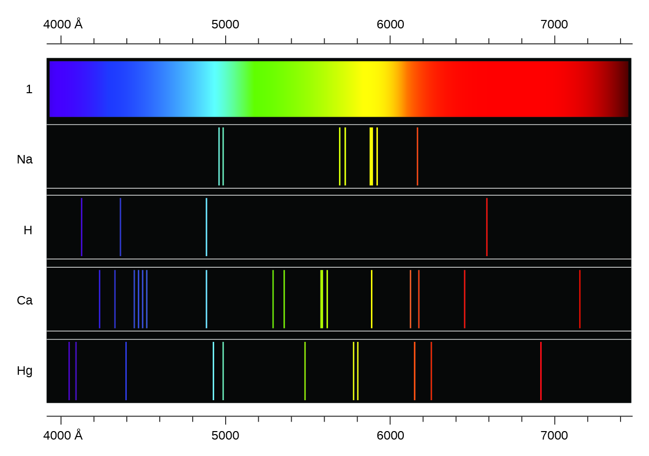
Figure \(\PageIndex{2}\): Line spectra of select gas. Compare the two types of emission spectra: continuous spectrum of white light (top) and the line spectra of the light from excited sodium, hydrogen, calcium, and mercury atoms.
The origin of discrete spectra in atoms and molecules was extremely puzzling to scientists in the late nineteenth century, since according to classical electromagnetic theory, only continuous spectra should be observed. Even more puzzling, in 1885, Johann Balmer was able to derive an empirical equation that related the four visible wavelengths of light emitted by hydrogen atoms to whole integers. That equation is the following one, in which k is a constant:
Other discrete lines for the hydrogen atom were found in the UV and IR regions. Johannes Rydberg generalized Balmer's work and developed an empirical formula that predicted all of hydrogen's emission lines, not just those restricted to the visible range, where, n1 and n2 are integers, n1 < n2, and \(R_∞\) is the Rydberg constant (1.097 × 10⁷ m−1).
Even in the late nineteenth century, spectroscopy was a very precise science, and so the wavelengths of hydrogen were measured to very high accuracy, which implied that the Rydberg constant could be determined very precisely as well. That such a simple formula as the Rydberg formula could account for such precise measurements seemed astounding at the time, but it was the eventual explanation for emission spectra by Neils Bohr in 1913 that ultimately convinced scientists to abandon classical physics and spurred the development of modern quantum mechanics.
Video \(\PageIndex{2}\): Emissions of electrons and the colors of elements.
Looking Further

Figure \(\PageIndex{3}\): Dr. Neil Degrasse Tyson. Photo Credit: NASA/Bill Ingalls
In his book, Astrophysics for People in a Hurry, Neil Degrasse Tyson talks about the origins of the universe and how we've used atomic spectroscopy and line spectra to determine what elements are present in various celestial bodies. Read versions of these essays by clicking the links below:
"Over the Rainbow" - A look at Spectroscopy and it's role in learning more about our universe.
"The Periodic Table of the Cosmos" - A look at the origin of the elements (from space!)
Behavior in the Microscopic World
We know how matter behaves in the macroscopic world—objects that are large enough to be seen by the naked eye follow the rules of classical physics. A billiard ball moving on a table will behave like a particle: It will continue in a straight line unless it collides with another ball or the table cushion, or is acted on by some other force (such as friction). The ball has a well-defined position and velocity (or a well-defined momentum, p = mv, defined by mass m and velocity v) at any given moment. In other words, the ball is moving in a classical trajectory. This is the typical behavior of a classical object.
When waves interact with each other, they show interference patterns that are not displayed by macroscopic particles such as the billiard ball. For example, interacting waves on the surface of water can produce interference patters similar to those shown on Figure \(\PageIndex{4}\). This is a case of wave behavior on the macroscopic scale, and it is clear that particles and waves are very different phenomena in the macroscopic realm.

Figure \(\PageIndex{4}\): An interference pattern on the water surface is formed by interacting waves. The waves are caused by reflection of water from the rocks. (credit: modification of work by Sukanto Debnath)
As technological improvements allowed scientists to probe the microscopic world in greater detail, it became increasingly clear by the 1920s that very small pieces of matter follow a different set of rules from those we observe for large objects. The unquestionable separation of waves and particles was no longer the case for the microscopic world.
One of the first people to pay attention to the special behavior of the microscopic world was Louis de Broglie. He asked the question: If electromagnetic radiation can have particle-like character, can electrons and other submicroscopic particles exhibit wavelike character? In his 1925 doctoral dissertation, de Broglie extended the wave–particle duality of light that Einstein used to resolve the photoelectric-effect paradox to material particles. He predicted that a particle with mass m and velocity v (that is, with linear momentum p) should also exhibit the behavior of a wave with a wavelength value λ, given by this expression in which h is the familiar Planck’s constant
\[\lambda=\dfrac{h}{mv}=\dfrac{h}{p} \label{6.4.1}\]
This is called the de Broglie wavelength. Unlike the other values of λ discussed in this chapter, the de Broglie wavelength is a characteristic of particles and other bodies, not electromagnetic radiation (note that this equation involves velocity [v, m/s], not frequency [ν, Hz]. Although these two symbols are identical, they mean very different things). Where Bohr had postulated the electron as being a particle orbiting the nucleus in quantized orbits, de Broglie argued that Bohr’s assumption of quantization can be explained if the electron is considered not as a particle, but rather as a circular standing wave such that only an integer number of wavelengths could fit exactly within the orbit (Figure \(\PageIndex{5}\)).
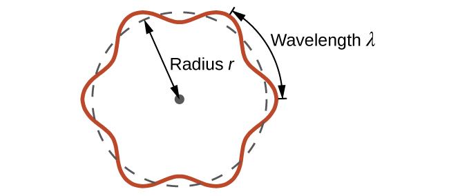
Figure \(\PageIndex{5}\): If an electron is viewed as a wave circling around the nucleus, an integer number of wavelengths must fit into the orbit for this standing wave behavior to be possible.
For a circular orbit of radius r, the circumference is 2πr, and so de Broglie’s condition is:
\[2πr=nλ \label{6.4.3}\]
with \(n=1,2,3,...\)
Since the de Broglie expression relates the wavelength to the momentum and, hence, velocity, this implies:
\[2πr=nλ=\dfrac{nh}{p}=\dfrac{nh}{mv}=\dfrac{nhr}{mvr}=\dfrac{nhr}{L} \label{6.4.3b}\]
This expression can be rearranged to give Bohr’s formula for the quantization of the angular momentum:
\[L=\dfrac{nh}{2π}=n \hbar \label{6.4.4}\]
Classical angular momentum L for a circular motion is equal to the product of the radius of the circle and the momentum of the moving particle p.
\[L=rp=rmv \;\;\; \text{(for a circular motion)} \label{6.4.5}\]
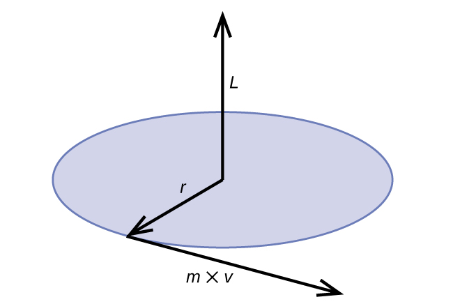
Figure \(\PageIndex{6}\): The diagram shows angular momentum for a circular motion.
Shortly after de Broglie proposed the wave nature of matter, two scientists at Bell Laboratories, C. J. Davisson and L. H. Germer, demonstrated experimentally that electrons can exhibit wavelike behavior by showing an interference pattern for electrons travelling through a regular atomic pattern in a crystal. The regularly spaced atomic layers served as slits, as used in other interference experiments. Since the spacing between the layers serving as slits needs to be similar in size to the wavelength of the tested wave for an interference pattern to form, Davisson and Germer used a crystalline nickel target for their “slits,” since the spacing of the atoms within the lattice was approximately the same as the de Broglie wavelengths of the electrons that they used. Figure \(\PageIndex{7}\) shows an interference pattern.
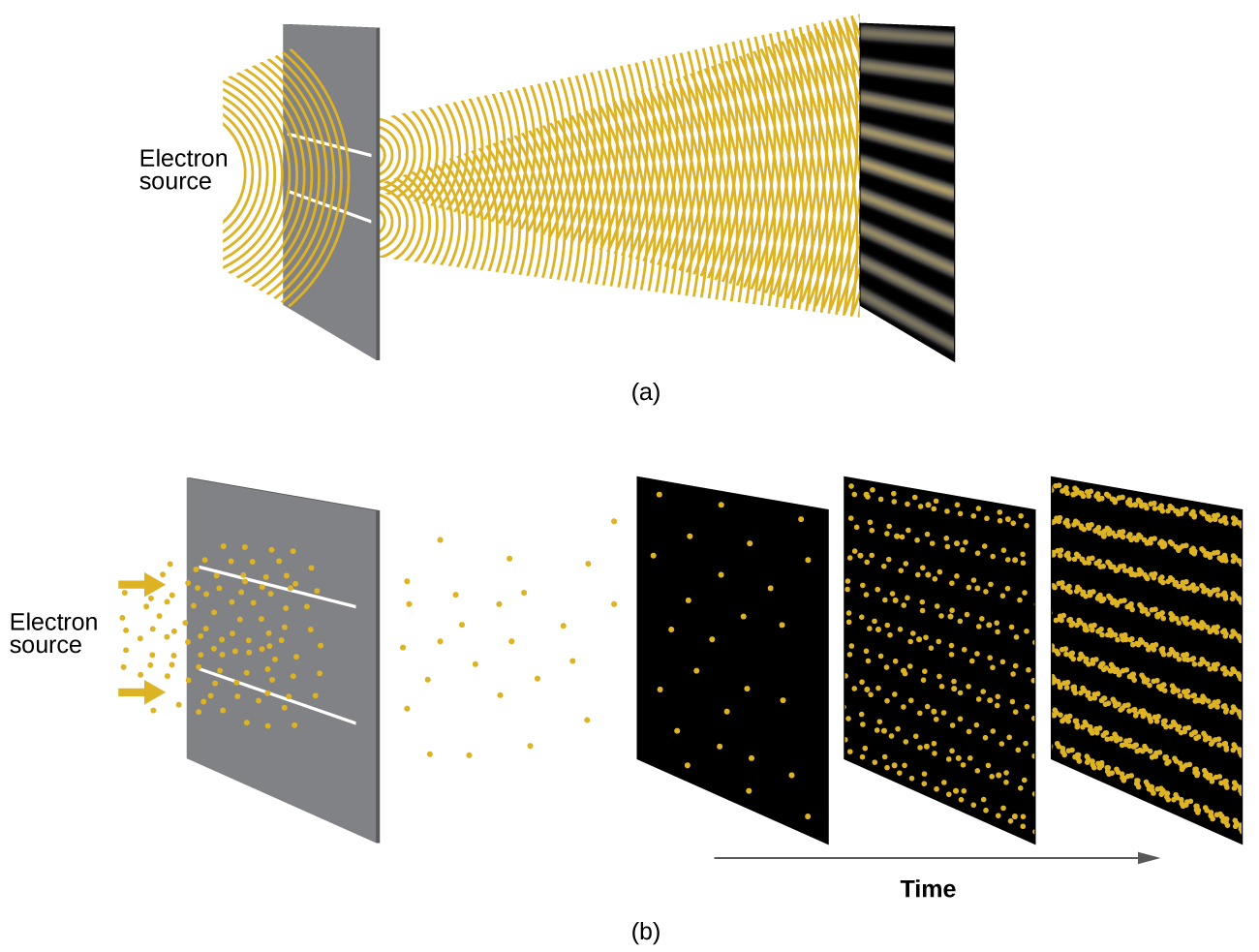
Figure \(\PageIndex{7}\): (a) The interference pattern for electrons passing through very closely spaced slits demonstrates that quantum particles such as electrons can exhibit wavelike behavior. (b) The experimental results illustrated here demonstrate the wave–particle duality in electrons. The electrons pass through very closely spaced slits, forming an interference pattern, with increasing numbers of electrons being recorded from the left image to the right. With only a few electrons recorded, it is clear that the electrons arrive as individual localized “particles,” but in a seemingly random pattern. As more electrons arrive, a wavelike interference pattern begins to emerge. Note that the probability of the final electron location is still governed by the wave-type distribution, even for a single electron, but it can be observed more easily if many electron collisions have been recorded.
The wave–particle duality of matter can be seen by observing what happens if electron collisions are recorded over a long period of time. Initially, when only a few electrons have been recorded, they show clear particle-like behavior, having arrived in small localized packets that appear to be random. As more and more electrons arrived and were recorded, a clear interference pattern that is the hallmark of wavelike behavior emerged. Thus, it appears that while electrons are small localized particles, their motion does not follow the equations of motion implied by classical mechanics, but instead it is governed by some type of a wave equation that governs a probability distribution even for a single electron’s motion. Thus the wave–particle duality first observed with photons is actually a fundamental behavior intrinsic to all quantum particles.
Video \(\PageIndex{3}\): View the Dr. Quantum – Double Slit Experiment cartoon for an easy-to-understand description of wave–particle duality and the associated experiments.
Example \(\PageIndex{1}\): Calculating the Wavelength of a Particle
If an electron travels at a velocity of 1.000 × 10⁷ m s–1 and has a mass of 9.109 × 10⁻²⁸ g, what is its wavelength?
Solution
We can use de Broglie’s equation to solve this problem, but we first must do a unit conversion of Planck’s constant. You learned earlier that 1 J = 1 kg m2/s2. Thus, we can write h = 6.626 × 10⁻³⁴ J s as 6.626 × 10⁻³⁴ kg m2/s.
&=\mathrm{\dfrac{6.626×10^{−34}\:kg\: m^2/s}{(9.109×10^{−31}\:kg)(1.000×10^7\:m/s)}}\\
&=\mathrm{7.274×10^{−11}\:m}
\end{align*}\)
This is a small value, but it is significantly larger than the size of an electron in the classical (particle) view. This size is the same order of magnitude as the size of an atom. This means that electron wavelike behavior is going to be noticeable in an atom.
Exercise \(\PageIndex{1}\)
Calculate the wavelength of a softball with a mass of 100 g traveling at a velocity of 35 m s–1, assuming that it can be modeled as a single particle.
- Answer
-
1.9 × 10⁻³⁴ m.
We never think of a thrown softball having a wavelength, since this wavelength is so small it is impossible for our senses or any known instrument to detect (strictly speaking, the wavelength of a real baseball would correspond to the wavelengths of its constituent atoms and molecules, which, while much larger than this value, would still be microscopically tiny). The de Broglie wavelength is only appreciable for matter that has a very small mass and/or a very high velocity.
Werner Heisenberg considered the limits of how accurately we can measure properties of an electron or other microscopic particles. He determined that there is a fundamental limit to how accurately one can measure both a particle’s position and its momentum simultaneously. The more accurately we measure the momentum of a particle, the less accurately we can determine its position at that time, and vice versa. This is summed up in what we now call the Heisenberg uncertainty principle: It is fundamentally impossible to determine simultaneously and exactly both the momentum and the position of a particle. For a particle of mass m moving with velocity vx in the x direction (or equivalently with momentum px), the product of the uncertainty in the position, Δx, and the uncertainty in the momentum, Δpx , must be greater than or equal to \(\dfrac{ℏ}{2}\) (recall that \(ℏ=\dfrac{h}{2π}\), the value of Planck’s constant divided by 2π).
\[Δx×Δp_x=(Δx)(mΔv)≥\dfrac{ℏ}{2}\]
This equation allows us to calculate the limit to how precisely we can know both the simultaneous position of an object and its momentum. For example, if we improve our measurement of an electron’s position so that the uncertainty in the position (Δx) has a value of, say, 1 pm (10–12 m, about 1% of the diameter of a hydrogen atom), then our determination of its momentum must have an uncertainty with a value of at least
\[\left [Δp=mΔv=\dfrac{h}{(2Δx)} \right ]=\mathrm{\dfrac{(1.055×10^{−34}\:kg\: m^2/s)}{(2×1×10^{−12}\:m)}=5×10^{−23}\:kg\: m/s.}\]
The value of ħ is not large, so the uncertainty in the position or momentum of a macroscopic object like a baseball is too insignificant to observe. However, the mass of a microscopic object such as an electron is small enough that the uncertainty can be large and significant.
It should be noted that Heisenberg’s uncertainty principle is not just limited to uncertainties in position and momentum, but it also links other dynamical variables. For example, when an atom absorbs a photon and makes a transition from one energy state to another, the uncertainty in the energy and the uncertainty in the time required for the transition are similarly related, as ΔE Δt ≥ \(\dfrac{ℏ}{2}\). As will be discussed later, even the vector components of angular momentum cannot all be specified exactly simultaneously.
Heisenberg’s principle imposes ultimate limits on what is knowable in science. The uncertainty principle can be shown to be a consequence of wave–particle duality, which lies at the heart of what distinguishes modern quantum theory from classical mechanics. Recall that the equations of motion obtained from classical mechanics are trajectories where, at any given instant in time, both the position and the momentum of a particle can be determined exactly. Heisenberg’s uncertainty principle implies that such a view is untenable in the microscopic domain and that there are fundamental limitations governing the motion of quantum particles. This does not mean that microscopic particles do not move in trajectories, it is just that measurements of trajectories are limited in their precision. In the realm of quantum mechanics, measurements introduce changes into the system that is being observed.
Video \(\PageIndex{4}\): VAn overview of the deBroglie wavelength.
Summary
Macroscopic objects act as particles. Microscopic objects (such as electrons) have properties of both a particle and a wave. Their exact trajectories cannot be determined. The quantum mechanical model of atoms describes the three-dimensional position of the electron in a probabilistic manner according to a mathematical function called a wavefunction, often denoted as ψ. Atomic wavefunctions are also called orbitals. The squared magnitude of the wavefunction describes the distribution of the probability of finding the electron in a particular region in space. Therefore, atomic orbitals describe the areas in an atom where electrons are most likely to be found.
Key Equation
- \(\lambda=\dfrac{h}{mv}=\dfrac{h}{p}\)
Contributors and Attributions
Paul Flowers (University of North Carolina - Pembroke), Klaus Theopold (University of Delaware) and Richard Langley (Stephen F. Austin State University) with contributing authors. Textbook content produced by OpenStax College is licensed under a Creative Commons Attribution License 4.0 license. Download for free at http://cnx.org/contents/85abf193-2bd...a7ac8df6@9.110).
- Adelaide Clark, Oregon Institute of Technology
- Crash Course Physics: Crash Course is a division of Complexly and videos are free to stream for educational purposes.
- Crash Course Astronomy: Crash Course is a division of Complexly and videos are free to stream for educational purposes.