Solutions 8
- Page ID
- 204086
\( \newcommand{\vecs}[1]{\overset { \scriptstyle \rightharpoonup} {\mathbf{#1}} } \)
\( \newcommand{\vecd}[1]{\overset{-\!-\!\rightharpoonup}{\vphantom{a}\smash {#1}}} \)
\( \newcommand{\dsum}{\displaystyle\sum\limits} \)
\( \newcommand{\dint}{\displaystyle\int\limits} \)
\( \newcommand{\dlim}{\displaystyle\lim\limits} \)
\( \newcommand{\id}{\mathrm{id}}\) \( \newcommand{\Span}{\mathrm{span}}\)
( \newcommand{\kernel}{\mathrm{null}\,}\) \( \newcommand{\range}{\mathrm{range}\,}\)
\( \newcommand{\RealPart}{\mathrm{Re}}\) \( \newcommand{\ImaginaryPart}{\mathrm{Im}}\)
\( \newcommand{\Argument}{\mathrm{Arg}}\) \( \newcommand{\norm}[1]{\| #1 \|}\)
\( \newcommand{\inner}[2]{\langle #1, #2 \rangle}\)
\( \newcommand{\Span}{\mathrm{span}}\)
\( \newcommand{\id}{\mathrm{id}}\)
\( \newcommand{\Span}{\mathrm{span}}\)
\( \newcommand{\kernel}{\mathrm{null}\,}\)
\( \newcommand{\range}{\mathrm{range}\,}\)
\( \newcommand{\RealPart}{\mathrm{Re}}\)
\( \newcommand{\ImaginaryPart}{\mathrm{Im}}\)
\( \newcommand{\Argument}{\mathrm{Arg}}\)
\( \newcommand{\norm}[1]{\| #1 \|}\)
\( \newcommand{\inner}[2]{\langle #1, #2 \rangle}\)
\( \newcommand{\Span}{\mathrm{span}}\) \( \newcommand{\AA}{\unicode[.8,0]{x212B}}\)
\( \newcommand{\vectorA}[1]{\vec{#1}} % arrow\)
\( \newcommand{\vectorAt}[1]{\vec{\text{#1}}} % arrow\)
\( \newcommand{\vectorB}[1]{\overset { \scriptstyle \rightharpoonup} {\mathbf{#1}} } \)
\( \newcommand{\vectorC}[1]{\textbf{#1}} \)
\( \newcommand{\vectorD}[1]{\overrightarrow{#1}} \)
\( \newcommand{\vectorDt}[1]{\overrightarrow{\text{#1}}} \)
\( \newcommand{\vectE}[1]{\overset{-\!-\!\rightharpoonup}{\vphantom{a}\smash{\mathbf {#1}}}} \)
\( \newcommand{\vecs}[1]{\overset { \scriptstyle \rightharpoonup} {\mathbf{#1}} } \)
\(\newcommand{\longvect}{\overrightarrow}\)
\( \newcommand{\vecd}[1]{\overset{-\!-\!\rightharpoonup}{\vphantom{a}\smash {#1}}} \)
\(\newcommand{\avec}{\mathbf a}\) \(\newcommand{\bvec}{\mathbf b}\) \(\newcommand{\cvec}{\mathbf c}\) \(\newcommand{\dvec}{\mathbf d}\) \(\newcommand{\dtil}{\widetilde{\mathbf d}}\) \(\newcommand{\evec}{\mathbf e}\) \(\newcommand{\fvec}{\mathbf f}\) \(\newcommand{\nvec}{\mathbf n}\) \(\newcommand{\pvec}{\mathbf p}\) \(\newcommand{\qvec}{\mathbf q}\) \(\newcommand{\svec}{\mathbf s}\) \(\newcommand{\tvec}{\mathbf t}\) \(\newcommand{\uvec}{\mathbf u}\) \(\newcommand{\vvec}{\mathbf v}\) \(\newcommand{\wvec}{\mathbf w}\) \(\newcommand{\xvec}{\mathbf x}\) \(\newcommand{\yvec}{\mathbf y}\) \(\newcommand{\zvec}{\mathbf z}\) \(\newcommand{\rvec}{\mathbf r}\) \(\newcommand{\mvec}{\mathbf m}\) \(\newcommand{\zerovec}{\mathbf 0}\) \(\newcommand{\onevec}{\mathbf 1}\) \(\newcommand{\real}{\mathbb R}\) \(\newcommand{\twovec}[2]{\left[\begin{array}{r}#1 \\ #2 \end{array}\right]}\) \(\newcommand{\ctwovec}[2]{\left[\begin{array}{c}#1 \\ #2 \end{array}\right]}\) \(\newcommand{\threevec}[3]{\left[\begin{array}{r}#1 \\ #2 \\ #3 \end{array}\right]}\) \(\newcommand{\cthreevec}[3]{\left[\begin{array}{c}#1 \\ #2 \\ #3 \end{array}\right]}\) \(\newcommand{\fourvec}[4]{\left[\begin{array}{r}#1 \\ #2 \\ #3 \\ #4 \end{array}\right]}\) \(\newcommand{\cfourvec}[4]{\left[\begin{array}{c}#1 \\ #2 \\ #3 \\ #4 \end{array}\right]}\) \(\newcommand{\fivevec}[5]{\left[\begin{array}{r}#1 \\ #2 \\ #3 \\ #4 \\ #5 \\ \end{array}\right]}\) \(\newcommand{\cfivevec}[5]{\left[\begin{array}{c}#1 \\ #2 \\ #3 \\ #4 \\ #5 \\ \end{array}\right]}\) \(\newcommand{\mattwo}[4]{\left[\begin{array}{rr}#1 \amp #2 \\ #3 \amp #4 \\ \end{array}\right]}\) \(\newcommand{\laspan}[1]{\text{Span}\{#1\}}\) \(\newcommand{\bcal}{\cal B}\) \(\newcommand{\ccal}{\cal C}\) \(\newcommand{\scal}{\cal S}\) \(\newcommand{\wcal}{\cal W}\) \(\newcommand{\ecal}{\cal E}\) \(\newcommand{\coords}[2]{\left\{#1\right\}_{#2}}\) \(\newcommand{\gray}[1]{\color{gray}{#1}}\) \(\newcommand{\lgray}[1]{\color{lightgray}{#1}}\) \(\newcommand{\rank}{\operatorname{rank}}\) \(\newcommand{\row}{\text{Row}}\) \(\newcommand{\col}{\text{Col}}\) \(\renewcommand{\row}{\text{Row}}\) \(\newcommand{\nul}{\text{Nul}}\) \(\newcommand{\var}{\text{Var}}\) \(\newcommand{\corr}{\text{corr}}\) \(\newcommand{\len}[1]{\left|#1\right|}\) \(\newcommand{\bbar}{\overline{\bvec}}\) \(\newcommand{\bhat}{\widehat{\bvec}}\) \(\newcommand{\bperp}{\bvec^\perp}\) \(\newcommand{\xhat}{\widehat{\xvec}}\) \(\newcommand{\vhat}{\widehat{\vvec}}\) \(\newcommand{\uhat}{\widehat{\uvec}}\) \(\newcommand{\what}{\widehat{\wvec}}\) \(\newcommand{\Sighat}{\widehat{\Sigma}}\) \(\newcommand{\lt}{<}\) \(\newcommand{\gt}{>}\) \(\newcommand{\amp}{&}\) \(\definecolor{fillinmathshade}{gray}{0.9}\)Q1:
The benefits of doing a geometry optimization is finding a mimimum energy state, which tends to be the most probable state a molecule exists in. This is in contrast to a molecular dynamics simulation which gives information about distributions of states. Geometry optimizations have the disadvantage of less information, but at a faster rate.
Q2:
The Born-Oppenheimer approximation separates the nuclear and electronic wavefunctions from one another, implying independence. This allows us to vary the coordinates of the nuclei and eletcrons independently of on another, which is what the geometry optimization procedure does. Without this approximation, we would have to consider the open problem of how nuclear motion affects electron motion. The one other important approximation that allows us to perform electronic calculations is the Hatree-Fock approximation which allows us to consider the electrons independently from one another.
Q3:
a). According to the Walsh diagram, 5 of the 13 molecular orbitals are occupied.
b). The sum is: = -12818-828.9-430.2-332.5-299.4 = -14709 kJ/mol
c). No, the basis set used Gaussians instead of the atomic orbital functions.
Q4:
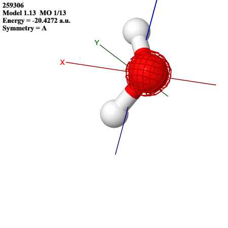
The lowest MO resembles an s orbital on oxygen:
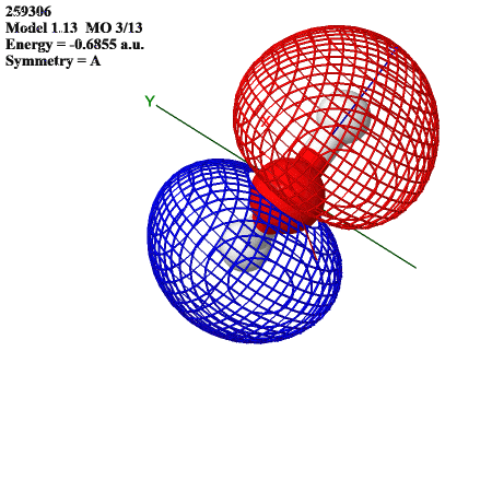
The HOMO resembles the s orbitals of the hydrogens overlapped with an oxygen p orbital:
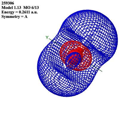
The LUMO resembles the s orbitals of hydrogens superimposed with the s orbital of oxygen, but with opposite phases:
Q5:
Water has \(C_{2v}\) point group symmetry, which means it has the symmetry operations E (identity), \(C_2\) (two fold rotationally symmetry, \(\sigma_v\) (xz plane reflection), and \(\sigma_v`\) (yz plane reflection).
| E | \(C_2\) (z) | \(\sigma_v\)(xz) | \(\sigma_v'\)(yz) | Linear, rotations | Quadratic | |
| \(A_1\) | 1 | 1 | 1 | 1 | z | \(x^2\), \(y^2\), \(z^2\) |
| \(A_2\) | 1 | 1 | -1 | -1 | \(R_z\) | xy |
| \(B_1\) | 1 | -1 | 1 | -1 | x, \(R_y\) | xz |
| \(B_2\) | 1 | -1 | -1 | 1 | y, \(R_x\) | yz |
Q6:
| MO | E | \(C_2\) (z) | \(\sigma_v\)(xz) | \(\sigma_v'\)(yz) | Representation |
| 1 | 1 | 1 | 1 | 1 | \(A_1\) |
| 2 | 1 | 1 | 1 | 1 | \(A_1\) |
| 3 | 1 | -1 | -1 | 1 | \(B_2\) |
| 4 | 1 | 1 | 1 | 1 | \(A_1\) |
| 5 | 1 | -1 | 1 | -1 | \(B_1\) |
| 6 | 1 | 1 | 1 | 1 | \(A_1\) |
| 7 | 1 | -1 | 1 | -1 | \(B_1\) |
Q7:
Look at the energy difference and equate it to \( E = \frac{hc}{\lambda}\) where E is energy, h is Planck's constant, c is the speed of light, and \(\\lambda\) is wavelength.
\(\Delta E = 163.8 - (-299.4) \) kJ/mol = 463 kJ/mol
Per molecule: 7.6944e-19 J
\(\lambda = \frac{hc}{E}\) = 2.583e-7 meters = 258 nm
Q8:
| Mode (energy in \(cm^{-1}\) | Type |
| .01 | translational |
| .01 | translational |
| 0 | translational |
| 482.86 | rotational |
| 535.39 | rotational |
| 624.6 | rotational |
| 1862.41 | vibrational |
| 3537.59 | vibrational |
| 3641.55 | vibrational |
Translatoinal < rotational < vibrational
Translational mode energies are lower than thermal energy (.049 \(cm^{-1}\))


