Acid-Base Titrations
- Page ID
- 221872
\( \newcommand{\vecs}[1]{\overset { \scriptstyle \rightharpoonup} {\mathbf{#1}} } \)
\( \newcommand{\vecd}[1]{\overset{-\!-\!\rightharpoonup}{\vphantom{a}\smash {#1}}} \)
\( \newcommand{\dsum}{\displaystyle\sum\limits} \)
\( \newcommand{\dint}{\displaystyle\int\limits} \)
\( \newcommand{\dlim}{\displaystyle\lim\limits} \)
\( \newcommand{\id}{\mathrm{id}}\) \( \newcommand{\Span}{\mathrm{span}}\)
( \newcommand{\kernel}{\mathrm{null}\,}\) \( \newcommand{\range}{\mathrm{range}\,}\)
\( \newcommand{\RealPart}{\mathrm{Re}}\) \( \newcommand{\ImaginaryPart}{\mathrm{Im}}\)
\( \newcommand{\Argument}{\mathrm{Arg}}\) \( \newcommand{\norm}[1]{\| #1 \|}\)
\( \newcommand{\inner}[2]{\langle #1, #2 \rangle}\)
\( \newcommand{\Span}{\mathrm{span}}\)
\( \newcommand{\id}{\mathrm{id}}\)
\( \newcommand{\Span}{\mathrm{span}}\)
\( \newcommand{\kernel}{\mathrm{null}\,}\)
\( \newcommand{\range}{\mathrm{range}\,}\)
\( \newcommand{\RealPart}{\mathrm{Re}}\)
\( \newcommand{\ImaginaryPart}{\mathrm{Im}}\)
\( \newcommand{\Argument}{\mathrm{Arg}}\)
\( \newcommand{\norm}[1]{\| #1 \|}\)
\( \newcommand{\inner}[2]{\langle #1, #2 \rangle}\)
\( \newcommand{\Span}{\mathrm{span}}\) \( \newcommand{\AA}{\unicode[.8,0]{x212B}}\)
\( \newcommand{\vectorA}[1]{\vec{#1}} % arrow\)
\( \newcommand{\vectorAt}[1]{\vec{\text{#1}}} % arrow\)
\( \newcommand{\vectorB}[1]{\overset { \scriptstyle \rightharpoonup} {\mathbf{#1}} } \)
\( \newcommand{\vectorC}[1]{\textbf{#1}} \)
\( \newcommand{\vectorD}[1]{\overrightarrow{#1}} \)
\( \newcommand{\vectorDt}[1]{\overrightarrow{\text{#1}}} \)
\( \newcommand{\vectE}[1]{\overset{-\!-\!\rightharpoonup}{\vphantom{a}\smash{\mathbf {#1}}}} \)
\( \newcommand{\vecs}[1]{\overset { \scriptstyle \rightharpoonup} {\mathbf{#1}} } \)
\(\newcommand{\longvect}{\overrightarrow}\)
\( \newcommand{\vecd}[1]{\overset{-\!-\!\rightharpoonup}{\vphantom{a}\smash {#1}}} \)
\(\newcommand{\avec}{\mathbf a}\) \(\newcommand{\bvec}{\mathbf b}\) \(\newcommand{\cvec}{\mathbf c}\) \(\newcommand{\dvec}{\mathbf d}\) \(\newcommand{\dtil}{\widetilde{\mathbf d}}\) \(\newcommand{\evec}{\mathbf e}\) \(\newcommand{\fvec}{\mathbf f}\) \(\newcommand{\nvec}{\mathbf n}\) \(\newcommand{\pvec}{\mathbf p}\) \(\newcommand{\qvec}{\mathbf q}\) \(\newcommand{\svec}{\mathbf s}\) \(\newcommand{\tvec}{\mathbf t}\) \(\newcommand{\uvec}{\mathbf u}\) \(\newcommand{\vvec}{\mathbf v}\) \(\newcommand{\wvec}{\mathbf w}\) \(\newcommand{\xvec}{\mathbf x}\) \(\newcommand{\yvec}{\mathbf y}\) \(\newcommand{\zvec}{\mathbf z}\) \(\newcommand{\rvec}{\mathbf r}\) \(\newcommand{\mvec}{\mathbf m}\) \(\newcommand{\zerovec}{\mathbf 0}\) \(\newcommand{\onevec}{\mathbf 1}\) \(\newcommand{\real}{\mathbb R}\) \(\newcommand{\twovec}[2]{\left[\begin{array}{r}#1 \\ #2 \end{array}\right]}\) \(\newcommand{\ctwovec}[2]{\left[\begin{array}{c}#1 \\ #2 \end{array}\right]}\) \(\newcommand{\threevec}[3]{\left[\begin{array}{r}#1 \\ #2 \\ #3 \end{array}\right]}\) \(\newcommand{\cthreevec}[3]{\left[\begin{array}{c}#1 \\ #2 \\ #3 \end{array}\right]}\) \(\newcommand{\fourvec}[4]{\left[\begin{array}{r}#1 \\ #2 \\ #3 \\ #4 \end{array}\right]}\) \(\newcommand{\cfourvec}[4]{\left[\begin{array}{c}#1 \\ #2 \\ #3 \\ #4 \end{array}\right]}\) \(\newcommand{\fivevec}[5]{\left[\begin{array}{r}#1 \\ #2 \\ #3 \\ #4 \\ #5 \\ \end{array}\right]}\) \(\newcommand{\cfivevec}[5]{\left[\begin{array}{c}#1 \\ #2 \\ #3 \\ #4 \\ #5 \\ \end{array}\right]}\) \(\newcommand{\mattwo}[4]{\left[\begin{array}{rr}#1 \amp #2 \\ #3 \amp #4 \\ \end{array}\right]}\) \(\newcommand{\laspan}[1]{\text{Span}\{#1\}}\) \(\newcommand{\bcal}{\cal B}\) \(\newcommand{\ccal}{\cal C}\) \(\newcommand{\scal}{\cal S}\) \(\newcommand{\wcal}{\cal W}\) \(\newcommand{\ecal}{\cal E}\) \(\newcommand{\coords}[2]{\left\{#1\right\}_{#2}}\) \(\newcommand{\gray}[1]{\color{gray}{#1}}\) \(\newcommand{\lgray}[1]{\color{lightgray}{#1}}\) \(\newcommand{\rank}{\operatorname{rank}}\) \(\newcommand{\row}{\text{Row}}\) \(\newcommand{\col}{\text{Col}}\) \(\renewcommand{\row}{\text{Row}}\) \(\newcommand{\nul}{\text{Nul}}\) \(\newcommand{\var}{\text{Var}}\) \(\newcommand{\corr}{\text{corr}}\) \(\newcommand{\len}[1]{\left|#1\right|}\) \(\newcommand{\bbar}{\overline{\bvec}}\) \(\newcommand{\bhat}{\widehat{\bvec}}\) \(\newcommand{\bperp}{\bvec^\perp}\) \(\newcommand{\xhat}{\widehat{\xvec}}\) \(\newcommand{\vhat}{\widehat{\vvec}}\) \(\newcommand{\uhat}{\widehat{\uvec}}\) \(\newcommand{\what}{\widehat{\wvec}}\) \(\newcommand{\Sighat}{\widehat{\Sigma}}\) \(\newcommand{\lt}{<}\) \(\newcommand{\gt}{>}\) \(\newcommand{\amp}{&}\) \(\definecolor{fillinmathshade}{gray}{0.9}\)Acid-Base titrations are usually used to find the amount of a known acidic or basic substance through acid base reactions. The analyte (titrand) is the solution with an unknown molarity. The reagent (titrant) is the solution with a known molarity that will react with the analyte.
Procedure
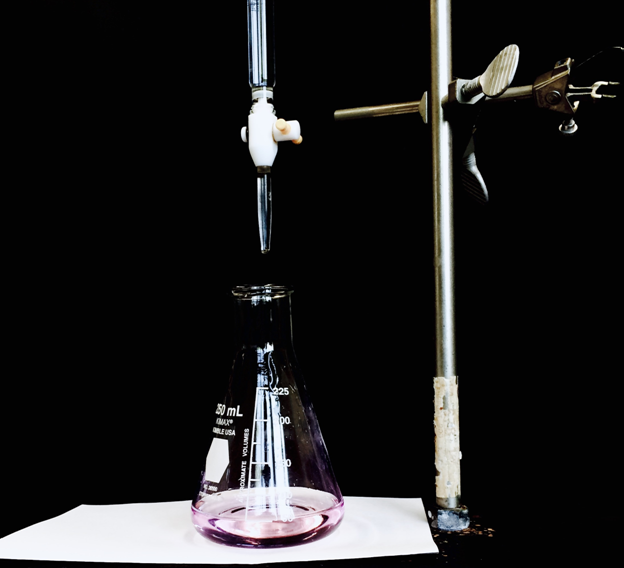
The analyte is prepared by dissolving the substance being studied into a solution. The solution is usually placed in a flask for titration. A small amount of indicator is then added into the flask along with the analyte. The reagent is usually placed in a burette and slowly added to the analyte and indicator mixture. The amount of reagent used is recorded when the indicator causes a change in the color of the solution.
Some titrations requires the solution to be boiled due to the \(CO_2\) created from the acid-base reaction. The \(CO_2\) forms carbonic acid (\(H_2CO_3\)) when dissolved in water that then acts as a buffer, reducing the accuracy of data. After boiling water, most of the \(CO_2\) will be removed from the solution allowing the solution to be titrated to a more accurate endpoint. The endpoint is the point where all of the analyte has be reacted with the reagent.
Indicator
A useful indicator has a strong color that changes quickly near its pKa. These traits are desirable so only a small amount of an indicator is needed. If a large amount of indicator is used, the indicator will effect the final pH, lowering the accuracy of the experiment. The indicator should also have a pKa value near the pH of the titration's endpoint. For example a analyte that is a weak base would require an indicator with a pKa less than 7. Choosing an indicator with a pKa near the endpoint's pH will also reduce error because the color change occurs sharply during the endpoint where the pH spikes, giving a more precise endpoint.

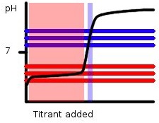
Figure 1: A Basic Titration Curve, The horizontal lines show the range of pH in which phenolphthalein (blue) and methyl orange (red) changes color. The middle line represents the pKa, while the two outer lines represent the end or start of the color changes. The peak and light blue highlights show the range in which the color changes will occur based on the amount of titrant added.
Notice that this reaction is between a weak acid and a strong base so phenolphthalein with a pKa of 9.1 would be a better choice than methyl orange with a pKa of 3.8. If in this reaction we were to use methyl orange as the indicator color changes would occur all throughout the region highlighted in pink. The data obtained would be hard to determine due to the large range of color change, and inaccurate as the color change does not even lie with the endpoint region. Phenolphthalein on the other hand changes color rapidly near the endpoint allowing for more accurate data to be gathered.


Multiply the volume of reagent added to get to the endpoint, with the molarity of the reagent to find the moles of reagent used. With the balanced equation of the acid-base reaction in question to find the moles of unknown substance. Then the original molarity can be calculated by dividing through with the initial volume.
For example an unknown molarity of \(HCl\) acts as the analyte. 50 mL of it is placed into a flask and a 0.1 M solution of \(NaOH\) will be the reagent. The endpoint is \(pH= 7\) so litmus, with a pKa of 6.5 is chosen. The color of the solution changes when 10 mL of 0.1 M \(NaOH\) is added.
The balanced neutralization reaction:
\[ HCl_{(aq)} + NaOH_{(aq)} \rightarrow H_2O_{(l)} + Na^+ + Cl^-\]
Or just the net ionic equation
\[H^+ + OH^- \rightarrow H_2O_{(l)} \]
The following equation can then be derived
\[ X= (0.1\; M \;\; NaOH) (10\;mL) \left(\dfrac{1\;L}{1000\; mL} \right) \left( \dfrac{1\;mol\; NaOH}{1\; mol \; OH^-} \right)\]
\[H^+ = X \;\; HCl\]
\(X = 0.0010 \;mol \;of\; HCl\)
The molarity is now easily solved for
\[ \dfrac{0.0010\; mol\; HCl}{0.050\; L} = 0.020\;M \;HCl\]
References
- Reactions of Acids and Bases in Analytical Chemistry. Hulanicki, A. and Masson, M.R. New York: Halsted Press, 1987.
- Aqueous Acid-Base Equilibria and Titrations. Levie, Robert De. New York : Oxford University Press, 1999.

