
4.7: Detection Limits
- Page ID
- 220682

\( \newcommand{\vecs}[1]{\overset { \scriptstyle \rightharpoonup} {\mathbf{#1}} } \)
\( \newcommand{\vecd}[1]{\overset{-\!-\!\rightharpoonup}{\vphantom{a}\smash {#1}}} \)
\( \newcommand{\id}{\mathrm{id}}\) \( \newcommand{\Span}{\mathrm{span}}\)
( \newcommand{\kernel}{\mathrm{null}\,}\) \( \newcommand{\range}{\mathrm{range}\,}\)
\( \newcommand{\RealPart}{\mathrm{Re}}\) \( \newcommand{\ImaginaryPart}{\mathrm{Im}}\)
\( \newcommand{\Argument}{\mathrm{Arg}}\) \( \newcommand{\norm}[1]{\| #1 \|}\)
\( \newcommand{\inner}[2]{\langle #1, #2 \rangle}\)
\( \newcommand{\Span}{\mathrm{span}}\)
\( \newcommand{\id}{\mathrm{id}}\)
\( \newcommand{\Span}{\mathrm{span}}\)
\( \newcommand{\kernel}{\mathrm{null}\,}\)
\( \newcommand{\range}{\mathrm{range}\,}\)
\( \newcommand{\RealPart}{\mathrm{Re}}\)
\( \newcommand{\ImaginaryPart}{\mathrm{Im}}\)
\( \newcommand{\Argument}{\mathrm{Arg}}\)
\( \newcommand{\norm}[1]{\| #1 \|}\)
\( \newcommand{\inner}[2]{\langle #1, #2 \rangle}\)
\( \newcommand{\Span}{\mathrm{span}}\) \( \newcommand{\AA}{\unicode[.8,0]{x212B}}\)
\( \newcommand{\vectorA}[1]{\vec{#1}} % arrow\)
\( \newcommand{\vectorAt}[1]{\vec{\text{#1}}} % arrow\)
\( \newcommand{\vectorB}[1]{\overset { \scriptstyle \rightharpoonup} {\mathbf{#1}} } \)
\( \newcommand{\vectorC}[1]{\textbf{#1}} \)
\( \newcommand{\vectorD}[1]{\overrightarrow{#1}} \)
\( \newcommand{\vectorDt}[1]{\overrightarrow{\text{#1}}} \)
\( \newcommand{\vectE}[1]{\overset{-\!-\!\rightharpoonup}{\vphantom{a}\smash{\mathbf {#1}}}} \)
\( \newcommand{\vecs}[1]{\overset { \scriptstyle \rightharpoonup} {\mathbf{#1}} } \)
\( \newcommand{\vecd}[1]{\overset{-\!-\!\rightharpoonup}{\vphantom{a}\smash {#1}}} \)
\(\newcommand{\avec}{\mathbf a}\) \(\newcommand{\bvec}{\mathbf b}\) \(\newcommand{\cvec}{\mathbf c}\) \(\newcommand{\dvec}{\mathbf d}\) \(\newcommand{\dtil}{\widetilde{\mathbf d}}\) \(\newcommand{\evec}{\mathbf e}\) \(\newcommand{\fvec}{\mathbf f}\) \(\newcommand{\nvec}{\mathbf n}\) \(\newcommand{\pvec}{\mathbf p}\) \(\newcommand{\qvec}{\mathbf q}\) \(\newcommand{\svec}{\mathbf s}\) \(\newcommand{\tvec}{\mathbf t}\) \(\newcommand{\uvec}{\mathbf u}\) \(\newcommand{\vvec}{\mathbf v}\) \(\newcommand{\wvec}{\mathbf w}\) \(\newcommand{\xvec}{\mathbf x}\) \(\newcommand{\yvec}{\mathbf y}\) \(\newcommand{\zvec}{\mathbf z}\) \(\newcommand{\rvec}{\mathbf r}\) \(\newcommand{\mvec}{\mathbf m}\) \(\newcommand{\zerovec}{\mathbf 0}\) \(\newcommand{\onevec}{\mathbf 1}\) \(\newcommand{\real}{\mathbb R}\) \(\newcommand{\twovec}[2]{\left[\begin{array}{r}#1 \\ #2 \end{array}\right]}\) \(\newcommand{\ctwovec}[2]{\left[\begin{array}{c}#1 \\ #2 \end{array}\right]}\) \(\newcommand{\threevec}[3]{\left[\begin{array}{r}#1 \\ #2 \\ #3 \end{array}\right]}\) \(\newcommand{\cthreevec}[3]{\left[\begin{array}{c}#1 \\ #2 \\ #3 \end{array}\right]}\) \(\newcommand{\fourvec}[4]{\left[\begin{array}{r}#1 \\ #2 \\ #3 \\ #4 \end{array}\right]}\) \(\newcommand{\cfourvec}[4]{\left[\begin{array}{c}#1 \\ #2 \\ #3 \\ #4 \end{array}\right]}\) \(\newcommand{\fivevec}[5]{\left[\begin{array}{r}#1 \\ #2 \\ #3 \\ #4 \\ #5 \\ \end{array}\right]}\) \(\newcommand{\cfivevec}[5]{\left[\begin{array}{c}#1 \\ #2 \\ #3 \\ #4 \\ #5 \\ \end{array}\right]}\) \(\newcommand{\mattwo}[4]{\left[\begin{array}{rr}#1 \amp #2 \\ #3 \amp #4 \\ \end{array}\right]}\) \(\newcommand{\laspan}[1]{\text{Span}\{#1\}}\) \(\newcommand{\bcal}{\cal B}\) \(\newcommand{\ccal}{\cal C}\) \(\newcommand{\scal}{\cal S}\) \(\newcommand{\wcal}{\cal W}\) \(\newcommand{\ecal}{\cal E}\) \(\newcommand{\coords}[2]{\left\{#1\right\}_{#2}}\) \(\newcommand{\gray}[1]{\color{gray}{#1}}\) \(\newcommand{\lgray}[1]{\color{lightgray}{#1}}\) \(\newcommand{\rank}{\operatorname{rank}}\) \(\newcommand{\row}{\text{Row}}\) \(\newcommand{\col}{\text{Col}}\) \(\renewcommand{\row}{\text{Row}}\) \(\newcommand{\nul}{\text{Nul}}\) \(\newcommand{\var}{\text{Var}}\) \(\newcommand{\corr}{\text{corr}}\) \(\newcommand{\len}[1]{\left|#1\right|}\) \(\newcommand{\bbar}{\overline{\bvec}}\) \(\newcommand{\bhat}{\widehat{\bvec}}\) \(\newcommand{\bperp}{\bvec^\perp}\) \(\newcommand{\xhat}{\widehat{\xvec}}\) \(\newcommand{\vhat}{\widehat{\vvec}}\) \(\newcommand{\uhat}{\widehat{\uvec}}\) \(\newcommand{\what}{\widehat{\wvec}}\) \(\newcommand{\Sighat}{\widehat{\Sigma}}\) \(\newcommand{\lt}{<}\) \(\newcommand{\gt}{>}\) \(\newcommand{\amp}{&}\) \(\definecolor{fillinmathshade}{gray}{0.9}\)The International Union of Pure and Applied Chemistry (IUPAC) defines a method’s detection limit as the smallest concentration or absolute amount of analyte that has a signal significantly larger than the signal from a suitable blank [IUPAC Compendium of Chemical Technology, Electronic Version]. Although our interest is in the amount of analyte, in this section we will define the detection limit in terms of the analyte’s signal. Knowing the signal you can calculate the analyte’s concentration, CA, or the moles of analyte, nA, using the equations
\[S_A = k_A C_A \text{ or } S_A = k_A n_A \nonumber\]
where k is the method’s sensitivity.
See Chapter 3 for a review of these equations.
Let’s translate the IUPAC definition of the detection limit into a mathematical form by letting Smb represent the average signal for a method blank, and letting \(\sigma_{mb}\) represent the method blank’s standard deviation. The null hypothesis is that the analyte is not present in the sample, and the alternative hypothesis is that the analyte is present in the sample. To detect the analyte, its signal must exceed Smb by a suitable amount; thus,
\[(S_A)_{DL} = S_{mb} \pm z \sigma_{mb} \label{4.1}\]
where \((S_A)_{DL}\) is the analyte’s detection limit.
If \(\sigma_{mb}\) is not known, we can replace it with smb; Equation \ref{4.1} then becomes
\[(S_A)_{DL} = S_{mb} \pm t s_{mb} \nonumber\]
You can make similar adjustments to other equations in this section. See, for example, Kirchner, C. J. “Estimation of Detection Limits for Environme tal Analytical Procedures,” in Currie, L. A. (ed) Detection in Analytical Chemistry: Importance, Theory, and Practice; American Chemical Society: Washington, D. C., 1988.
The value we choose for z depends on our tolerance for reporting the analyte’s concentration even if it is absent from the sample (a type 1 error). Typically, z is set to three, which, from Appendix 3, corresponds to a probability, \(\alpha\), of 0.00135. As shown in Figure \(\PageIndex{1}\)a, there is only a 0.135% probability of detecting the analyte in a sample that actually is analyte-free.
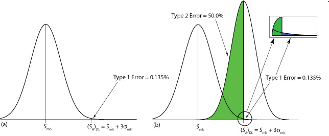
A detection limit also is subject to a type 2 error in which we fail to find evidence for the analyte even though it is present in the sample. Consider, for example, the situation shown in Figure \(\PageIndex{1}\)b where the signal for a sample that contains the analyte is exactly equal to (SA)DL. In this case the probability of a type 2 error is 50% because half of the sample’s possible signals are below the detection limit. We correctly detect the analyte at the IUPAC detection limit only half the time. The IUPAC definition for the detection limit is the smallest signal for which we can say, at a significance level of \(\alpha\), that an analyte is present in the sample; however, failing to detect the analyte does not mean it is not present in the sample.
The detection limit often is represented, particularly when discussing public policy issues, as a distinct line that separates detectable concentrations of analytes from concentrations we cannot detect. This use of a detection limit is incorrect [Rogers, L. B. J. Chem. Educ. 1986, 63, 3–6]. As suggested by Figure \(\PageIndex{1}\), for an analyte whose concentration is near the detection limit there is a high probability that we will fail to detect the analyte.
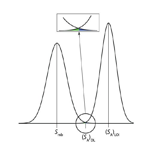
An alternative expression for the detection limit, the limit of identification, minimizes both type 1 and type 2 errors [Long, G. L.; Winefordner, J. D. Anal. Chem. 1983, 55, 712A–724A]. The analyte’s signal at the limit of identification, (SA)LOI, includes an additional term, \(z \sigma_A\), to account for the distribution of the analyte’s signal.
\[(S_A)_\text{LOI} = (S_A)_\text{DL} + z \sigma_A = S_{mb} + z \sigma_{mb} + z \sigma_A \nonumber\]
As shown in Figure \(\PageIndex{2}\), the limit of identification provides an equal probability of a type 1 and a type 2 error at the detection limit. When the analyte’s concentration is at its limit of identification, there is only a 0.135% probability that its signal is indistinguishable from that of the method blank.
The ability to detect the analyte with confidence is not the same as the ability to report with confidence its concentration, or to distinguish between its concentration in two samples. For this reason the American Chemical Society’s Committee on Environmental Analytical Chemistry recommends the limit of quantitation, (SA)LOQ [“Guidelines for Data Acquisition and Data Quality Evaluation in Environmental Chemistry,” Anal. Chem. 1980, 52, 2242–2249 ].
\[(S_A)_\text{LOQ} = S_{mb} + 10 \sigma_{mb} \nonumber\]