
3: The Rise of Quantum Mechanics (Lecture)
- Page ID
- 198568
\( \newcommand{\vecs}[1]{\overset { \scriptstyle \rightharpoonup} {\mathbf{#1}} } \)
\( \newcommand{\vecd}[1]{\overset{-\!-\!\rightharpoonup}{\vphantom{a}\smash {#1}}} \)
\( \newcommand{\id}{\mathrm{id}}\) \( \newcommand{\Span}{\mathrm{span}}\)
( \newcommand{\kernel}{\mathrm{null}\,}\) \( \newcommand{\range}{\mathrm{range}\,}\)
\( \newcommand{\RealPart}{\mathrm{Re}}\) \( \newcommand{\ImaginaryPart}{\mathrm{Im}}\)
\( \newcommand{\Argument}{\mathrm{Arg}}\) \( \newcommand{\norm}[1]{\| #1 \|}\)
\( \newcommand{\inner}[2]{\langle #1, #2 \rangle}\)
\( \newcommand{\Span}{\mathrm{span}}\)
\( \newcommand{\id}{\mathrm{id}}\)
\( \newcommand{\Span}{\mathrm{span}}\)
\( \newcommand{\kernel}{\mathrm{null}\,}\)
\( \newcommand{\range}{\mathrm{range}\,}\)
\( \newcommand{\RealPart}{\mathrm{Re}}\)
\( \newcommand{\ImaginaryPart}{\mathrm{Im}}\)
\( \newcommand{\Argument}{\mathrm{Arg}}\)
\( \newcommand{\norm}[1]{\| #1 \|}\)
\( \newcommand{\inner}[2]{\langle #1, #2 \rangle}\)
\( \newcommand{\Span}{\mathrm{span}}\) \( \newcommand{\AA}{\unicode[.8,0]{x212B}}\)
\( \newcommand{\vectorA}[1]{\vec{#1}} % arrow\)
\( \newcommand{\vectorAt}[1]{\vec{\text{#1}}} % arrow\)
\( \newcommand{\vectorB}[1]{\overset { \scriptstyle \rightharpoonup} {\mathbf{#1}} } \)
\( \newcommand{\vectorC}[1]{\textbf{#1}} \)
\( \newcommand{\vectorD}[1]{\overrightarrow{#1}} \)
\( \newcommand{\vectorDt}[1]{\overrightarrow{\text{#1}}} \)
\( \newcommand{\vectE}[1]{\overset{-\!-\!\rightharpoonup}{\vphantom{a}\smash{\mathbf {#1}}}} \)
\( \newcommand{\vecs}[1]{\overset { \scriptstyle \rightharpoonup} {\mathbf{#1}} } \)
\( \newcommand{\vecd}[1]{\overset{-\!-\!\rightharpoonup}{\vphantom{a}\smash {#1}}} \)
\(\newcommand{\avec}{\mathbf a}\) \(\newcommand{\bvec}{\mathbf b}\) \(\newcommand{\cvec}{\mathbf c}\) \(\newcommand{\dvec}{\mathbf d}\) \(\newcommand{\dtil}{\widetilde{\mathbf d}}\) \(\newcommand{\evec}{\mathbf e}\) \(\newcommand{\fvec}{\mathbf f}\) \(\newcommand{\nvec}{\mathbf n}\) \(\newcommand{\pvec}{\mathbf p}\) \(\newcommand{\qvec}{\mathbf q}\) \(\newcommand{\svec}{\mathbf s}\) \(\newcommand{\tvec}{\mathbf t}\) \(\newcommand{\uvec}{\mathbf u}\) \(\newcommand{\vvec}{\mathbf v}\) \(\newcommand{\wvec}{\mathbf w}\) \(\newcommand{\xvec}{\mathbf x}\) \(\newcommand{\yvec}{\mathbf y}\) \(\newcommand{\zvec}{\mathbf z}\) \(\newcommand{\rvec}{\mathbf r}\) \(\newcommand{\mvec}{\mathbf m}\) \(\newcommand{\zerovec}{\mathbf 0}\) \(\newcommand{\onevec}{\mathbf 1}\) \(\newcommand{\real}{\mathbb R}\) \(\newcommand{\twovec}[2]{\left[\begin{array}{r}#1 \\ #2 \end{array}\right]}\) \(\newcommand{\ctwovec}[2]{\left[\begin{array}{c}#1 \\ #2 \end{array}\right]}\) \(\newcommand{\threevec}[3]{\left[\begin{array}{r}#1 \\ #2 \\ #3 \end{array}\right]}\) \(\newcommand{\cthreevec}[3]{\left[\begin{array}{c}#1 \\ #2 \\ #3 \end{array}\right]}\) \(\newcommand{\fourvec}[4]{\left[\begin{array}{r}#1 \\ #2 \\ #3 \\ #4 \end{array}\right]}\) \(\newcommand{\cfourvec}[4]{\left[\begin{array}{c}#1 \\ #2 \\ #3 \\ #4 \end{array}\right]}\) \(\newcommand{\fivevec}[5]{\left[\begin{array}{r}#1 \\ #2 \\ #3 \\ #4 \\ #5 \\ \end{array}\right]}\) \(\newcommand{\cfivevec}[5]{\left[\begin{array}{c}#1 \\ #2 \\ #3 \\ #4 \\ #5 \\ \end{array}\right]}\) \(\newcommand{\mattwo}[4]{\left[\begin{array}{rr}#1 \amp #2 \\ #3 \amp #4 \\ \end{array}\right]}\) \(\newcommand{\laspan}[1]{\text{Span}\{#1\}}\) \(\newcommand{\bcal}{\cal B}\) \(\newcommand{\ccal}{\cal C}\) \(\newcommand{\scal}{\cal S}\) \(\newcommand{\wcal}{\cal W}\) \(\newcommand{\ecal}{\cal E}\) \(\newcommand{\coords}[2]{\left\{#1\right\}_{#2}}\) \(\newcommand{\gray}[1]{\color{gray}{#1}}\) \(\newcommand{\lgray}[1]{\color{lightgray}{#1}}\) \(\newcommand{\rank}{\operatorname{rank}}\) \(\newcommand{\row}{\text{Row}}\) \(\newcommand{\col}{\text{Col}}\) \(\renewcommand{\row}{\text{Row}}\) \(\newcommand{\nul}{\text{Nul}}\) \(\newcommand{\var}{\text{Var}}\) \(\newcommand{\corr}{\text{corr}}\) \(\newcommand{\len}[1]{\left|#1\right|}\) \(\newcommand{\bbar}{\overline{\bvec}}\) \(\newcommand{\bhat}{\widehat{\bvec}}\) \(\newcommand{\bperp}{\bvec^\perp}\) \(\newcommand{\xhat}{\widehat{\xvec}}\) \(\newcommand{\vhat}{\widehat{\vvec}}\) \(\newcommand{\uhat}{\widehat{\uvec}}\) \(\newcommand{\what}{\widehat{\wvec}}\) \(\newcommand{\Sighat}{\widehat{\Sigma}}\) \(\newcommand{\lt}{<}\) \(\newcommand{\gt}{>}\) \(\newcommand{\amp}{&}\) \(\definecolor{fillinmathshade}{gray}{0.9}\)A brief recap of Lecture 2:
Classical mechanics is unable to explain certain phenomena observed in nature. We will discuss three of these phenomena. Last lecture we discussed the photoelectron effect and introduces hydrogen atom emission, the last two of these phenomena (to accompany blackbody radiation discussed in Lecture 1). There are many more example of classical mechanics breakdown, but these are the historical and traditional three that are introduced in quantum classes.
The photoelectron effect has several experimental observations that break with classical predictions. Einstein proposed a solution that light is quantized given by the formula
\[E = h \nu \nonumber\]
where each quantum of light is called a photon. And the energy is proportional to its frequency \(\nu\)). This was an impressive argument in that it said light is not always a wave, but can be a particle. As we will see in todays' lecture, this duality also applies to matter.
The classical picture of the hydrogen emission is that a broad continuum of "photons" would be absorbed by matter (e.g., hydrogen atoms). Experimentally, "lines" are observed instead, suggesting that matter is "quantized" too. This is the topic of today's lecture.
Light Waves
Many of the properties of light (e.g., surface of water or acoustics) including reflection, refraction, diffraction, and interference can be explained, both qualitatively and quantitatively, in terms of light viewed as a wave.
The amplitudes of waves add. Constructive interference is obtained when identical waves are in phase and destructive interference occurs when identical waves are exactly out of phase, or shifted by half a wavelength.
Quantum Matter Waves
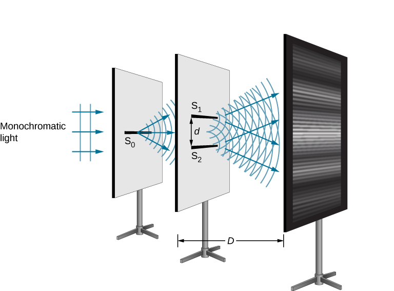
Continuing with our analysis of experiments that lead to the new quantum theory, we now look at the phenomenon of electron diffraction. It is well-known that light has the ability to diffract around objects in its path, leading to an interference pattern that is particular to the object. This is, in fact, how holography works (the interference pattern is created by allowing the diffracted light to interfere with the original beam so that the hologram can be viewed by shining the original beam on the image). A simple illustration of diffraction is the Young double slit experiment pictured below:
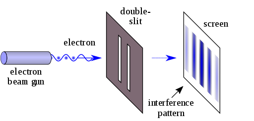
Amazingly, if electrons are used instead of light in the double-slit experiment, and a fluorescent screen is used, one finds the same kind of interference pattern! This is shown in the electron double-slit diffraction pattern below:
Obviously, classical mechanics is not able to predict such a result. If the electrons are treated as classical particles, one would predict an intensity pattern corresponding to particles that can pass through one slit or the other, landing on the screen directly opposite the slit (i.e., no intensity maximum at the center of the screen):
Through such experiments, the idea that electrons can behave as waves, creating interference patterns normally associated with light, is now well-established. The fact that particles can behave as waves but also as particles, depending on which experiment you perform on them, is known as the particle-wave duality.
Deriving the De Broglie Wavelength
De Broglie derived his equation using well established theories through the following series of substitutions:
1. De Broglie first used Einstein's famous equation relating matter and energy:
\[ E = mc^2 \label{0}\]
with
- \(E\) = energy,
- \(m\) = mass,
- \(c\) = speed of light
2. Using Planck's theory which states every quantum of a wave has a discrete amount of energy given by Planck's equation:
\[ E= h \nu \label{1}\]
with
- \(E\) = energy,
- \(h\) = Plank's constant (6.62607 x 10⁻³⁴ J s),
- \(\nu\)= frequency
3. Since de Broglie believed particles and wave have the same traits, he hypothesized that the two energies would be equal:
\[ mc^2 = h\nu \label{2}\]
4. Because real particles do not travel at the speed of light, De Broglie submitted velocity (\(v\)) for the speed of light (\(c\)).
\[ mv^2 = h\nu \label{3}\]
5. Through the equation \(\lambda\), de Broglie substituted \( v/\lambda\) for \(\nu\) and arrived at the final expression that relates wavelength and particle with speed.
\[ mv^2 = \dfrac{hv}{\lambda} \label{4}\]
Hence:
\[ \lambda = \dfrac{hv}{mv^2} = \dfrac{h}{mv} \label{5} \]
A majority of Wave-Particle Duality problems are simple plug and chug via Equation \ref{5} with some variation of canceling out units
Example \(\PageIndex{1}\)
Find the de Broglie wavelength for an electron moving at the speed of \(5.0 \times 10^6\; m/s\) (mass of an electron is \(9.1 \times 10^{-31}\; kg\)).
- Answer:
- This is a straightforward application of the de Broglie wavelength equation. \[ \lambda = \dfrac{h}{p}= \dfrac{h}{mv} =\dfrac{6.63 \times 10^{-34}\; J \cdot s}{(9.1 \times 10^{-31} \; kg)(5.0 \times 10^6\, m/s)}= 1.46 \times 10^{-10}\;m\]
Size matters in Quantum Mechanics
To effectively diffract a wave, the wavelength of the wave must be comparable to the dimensions of the diffraction device!
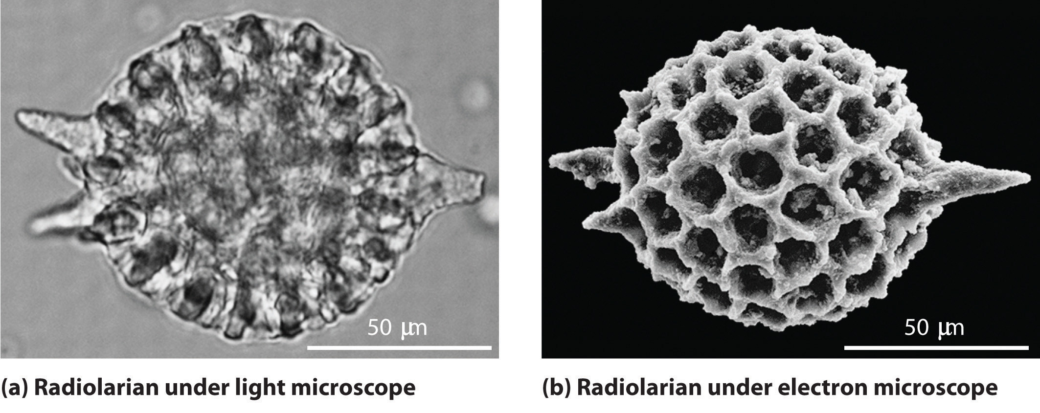
Although we still usually think of electrons as particles, the wave nature of electrons is employed in an electron microscope, which has revealed most of what we know about the microscopic structure of living organisms and materials. Because the wavelength of an electron beam is much shorter than the wavelength of a beam of visible light, this instrument can resolve smaller details than a light microscope can:
Hydrogen Atoms Models
Model 1: The Rutherford model
The Coulomb force that exists between oppositely charge particles means that a positive nucleus and negative electrons should attract each other, and the atom should collapse. To prevent the collapse, the electron was postulated to be orbiting the positive nucleus. The Coulomb force (discussed below) is used to change the direction of the velocity, just as a string pulls a ball in a circular orbit around your head or the gravitational force holds the moon in orbit around the Earth. The origin for this hypothesis that suggests this perspective is plausible is the similarity of the gravity and Coulombic interactions. The expression for the force of gravity between two masses (Newton's Law of gravity) is
\[F_{gravity} \propto \dfrac{m_1m_2}{r^2}\label{1.8.1}\]
with
- \(m_1\) and \(m_2\) representing the mass of object 1 and 2, respectively and
- \(r\) representing the distance between the objects centers
The expression for the Coulomb force between two charged species is
\[F_{Coulomb} \propto \dfrac{Q_1Q_2}{r^2}\label{1.8.2}\]
with
- \(Q_1\) and \(Q_2\) representing the charge of object 1 and 2, respectively and
- \(r\) representing the distance between the objects centers
However this analogy has a problem too. An electron going around in a circle is constantly being accelerated because its velocity vector is changing. A charged particle that is being accelerated emits radiation. This property is essentially how a radio transmitter works. A power supply drives electrons up and down a wire and thus transmits energy (electromagnetic radiation) that your radio receiver picks up. The radio then plays the music for you that is encoded in the waveform of the radiated energy.

Model 2A: The Classical Bohr Atom (Electron as a Particle)
The Bohr model is an early attempt to predict the allowed energies for single-electron atoms such as \(H\), \(He^{+}\), \(Li^{2+}\), \(Be^{3+}\), etc. Although Bohr's reasoning relies on classical concepts and hence, is not a correct explanation, the reasoning is interesting, and so we examine this model for its historical significance.
In 1911, Niels Bohr introduced his theory on the hydrogen atom. It assumed three main points.
- Electrons move in circular orbitals.
- Electrons are confined by Coulombic force
- The wave nature of particles leads to quantization of energy levels of an atom.
Calculation of the orbits requires two assumptions.
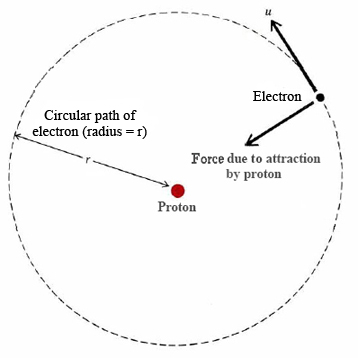
Assumption 1: The electron is held in a circular orbit by electrostatic attraction
The Coulombic force of the attraction between the proton and electron can be written as
\[F_{coulombic} = \dfrac {e^2}{4\pi \epsilon_0 r^2} \label{BHeq1}\]
where \(e\) is the charge of the electron, \(\epsilon_0\) is the perimittivity of free space, and \(r\) is the radius of the electron orbit. The Coulombic force is counterbalanced by centrifugal force
\[F_{centrifugal} = m_e \cdot \dfrac {v^2}{r} \label{BHeq2}\]
where \(m_e\) is the mass of the electron, and \(v\) is the speed of the electron.
Assumption 2: The angular momentum is quantized
Bohr assumed that angular momentum of the electron was quantized (more below)
\[L = m_e vr = \dfrac {nh}{2\pi} \label{BH0}\]
Setting Equations \ref{BHeq1} and \ref{BHeq2} equal to each other and solving for \(r\) and introducing Equation \ref{BH0}, the radius of the electron's orbit, gives
\[r = \dfrac {\epsilon_0 h^2 n^2}{\pi m_e e^2}\]
The symbol \(\hbar\) is more commonly used in quantum mechanics, which is equivalent to \(\dfrac {h}{2\pi}\), so the equation for the radius of the orbit can be written as
\[r = \dfrac {4\pi \epsilon_0 \hbar^2 n^2}{m_e e^2} \label{BA1}\]
Using \(n\) = \(1\), you get an \(r\) value of \(5.29 \times 10^{-11} m\). So equation \ref{BA1} can be rewritten as
\[r = n^2 a_o \label{BA2}\]
where
\[a_o = \dfrac {4\pi \epsilon_0 \hbar^2 }{m_e e^2} = 5.29 \times 10^{-11} m\]
\(a_o\) is often called the Bohr radius (i.e. radius of an unexcited hydrogen atom).
Example \(\PageIndex{2}\): Quantized ORbits
A hydrogen atom is in its first excited state (\(n = 2\)). Using the Bohr theory of the atom, calculate the radius of the orbit.
- Solution
- This is a straightforward application of Equation \ref{BA2} with \(n=2\). \[ r_2 = 2^2 a_o = 4 a_o = 4 (5.29 \times 10^{-11} m) = 2.12 \times 10^{-10}\;m\] The dimensions of atoms are often expressed in nanometers (\(1\, nm = 10^{-9}\, m\)) or angstroms (\(1\, Å = 10^{-10}\,m\)). So the radius of this excited hydrogen atom is 0.212 nm or 2.12 Å.
The total energy of any system can be denoted by
\[E = T + V\]
the summation of the systems kinetic and potential energy, respectively. Setting the system to be an electron allows for the total energy of the electron in a Hydrogen atom to be calculated. In this case, the kinetic energy is
\[T = \dfrac{ m_e v^2}{2}\]
and
\[V = - \dfrac {e^2}{4\pi \epsilon_0 r}.\]
Thus,
\[E = \dfrac{m_e v^2}{2} - \dfrac {e^2}{4\pi \epsilon_0 r}\]
By substituting \(m_e v^2\) by equating \(F_{coulombic}\) and \(F_{centrifugal}\), and plugging in the Bohr radius for \(r\) (Equation \(\ref{BA1}\)) results in
\[E_n = \dfrac {-m_e e^4}{8\epsilon^2_0 h^2} \cdot \dfrac {1}{n^2} \label{R1}\]
or
\[E_n = -R \dfrac {1}{n^2} \label{BA5}\]
where \(R\) is the Rydberg constant, which is sometimes referred to as \(R_\infty\) or \(R_H\).
The energy of an orbital is negative indicating that the negatively charged electron is bound by the positive nucleus, and therefore it requires energy to free the electron from the atom. When assuming the nuclear mass is infinite compared to the mass of the electron, the value of \(R_\infty\) is \(109737 cm^{-1}\) or \(13.6\, eV\). When properly taking the nuclear mass into account, \(R_H\) is \(109677 cm^{-1}\).
Example \(\PageIndex{3}\): Quantized Energies
A hydrogen atom is in its first excited state (\(n = 2\)). Using the Bohr theory of the atom, calculate the energy of the electron in this orbit.
- Solution
- This is a straightforward application of Equation \ref{BA5} with \(n=2\). \[ E_n = -R \dfrac {1}{2^2} = \dfrac{R}{4} = \dfrac{13.6\, eV}{4} = 3.4 \,eV\] The electron is higher in the Coloumbic well and hence requires less energy to remove.
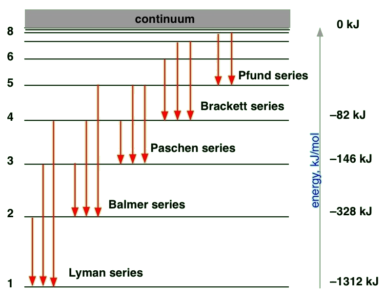
State-to-state Transitions
A Hydrogen atom emits radiation when the e- makes a transition from a higher energy orbit (state, orbital) to a lower one. Alternatively, the electron can absorb a photon by "jumping" (changing) from one quantum state to another.
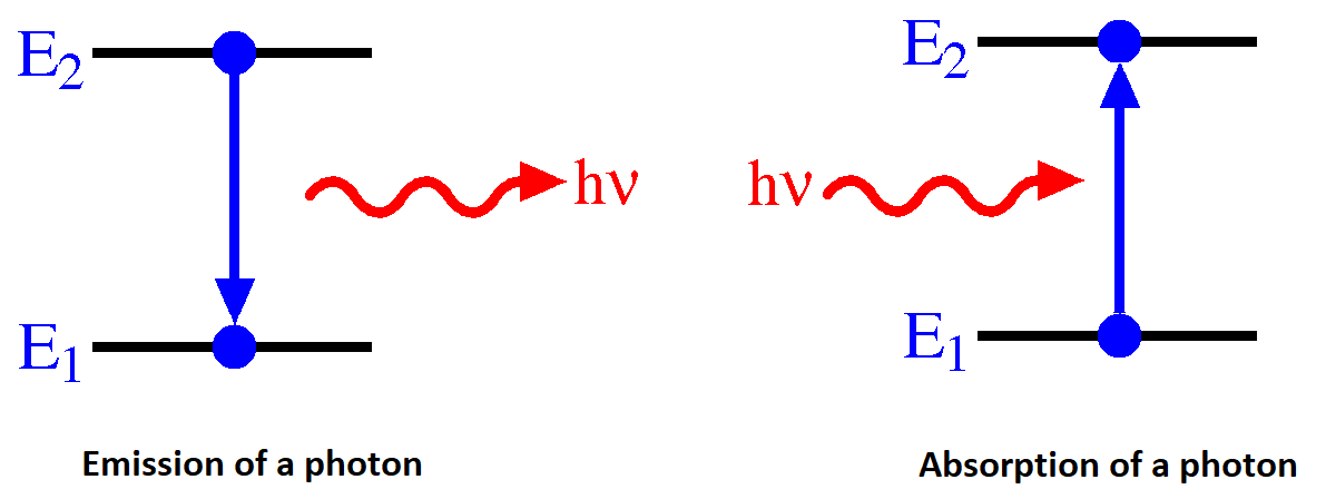
For emission, the conservation of energy in the absorption transition would look like
\[ E_{n_i} + hv = E_{n_f} \]
and similarly for emission transition
\[ E_{n_i} - hv = E_{n_f} \label{emission} \]
where the energy of the state is a function of the \(n_i\) and \(n_f\) integers for the initial and final states. For emission, we can now expand Equation \ref{emission} using Equation \ref{R1}
\[\nu=\dfrac{E_{n_i}-E_{n_f}}{h}=\dfrac{e^4 m_e}{8\epsilon_{0}^{2} h^3}\left ( \dfrac{1}{n_{f}^{2}}-\dfrac{1}{n_{i}^{2}}\right ) \label{1.8.23}\]
We can now identify the Rydberg constant \(R_H\) and it is not phenomenological, but can be expressed in terms of basic physical constants on the right hand side of Equation \(\ref{1.8.23}\)
\[ \begin{align*} R_H &= \dfrac {me^4}{8 \epsilon ^2_0 h^3 } \\[4pt] &\approx 2.19 \times 10^{-18} J \end{align*}\]
and in terms of wavenumbers using the \(c=\lambda \nu\) relationship
\[ \begin{align*} R_H &= \dfrac {me^4}{8 \epsilon ^2_0 h^3c } \\[4pt] &\approx 109,737 \,cm^{-1} \end{align*}\]
A demo of both wavelength and particle like Bohr atoms: http://www.walter-fendt.de/html5/phe...hrmodel_en.htm
Continued in Lecture 4...