Time-Correlation Functions

Last updated
Save as PDF

Page ID: 78480

\( \newcommand{\vecs}[1]{\overset { \scriptstyle \rightharpoonup} {\mathbf{#1}} } \) \( \newcommand{\vecd}[1]{\overset{-\!-\!\rightharpoonup}{\vphantom{a}\smash {#1}}} \)\(\newcommand{\id}{\mathrm{id}}\) \( \newcommand{\Span}{\mathrm{span}}\) \( \newcommand{\kernel}{\mathrm{null}\,}\) \( \newcommand{\range}{\mathrm{range}\,}\) \( \newcommand{\RealPart}{\mathrm{Re}}\) \( \newcommand{\ImaginaryPart}{\mathrm{Im}}\) \( \newcommand{\Argument}{\mathrm{Arg}}\) \( \newcommand{\norm}[1]{\| #1 \|}\) \( \newcommand{\inner}[2]{\langle #1, #2 \rangle}\) \( \newcommand{\Span}{\mathrm{span}}\) \(\newcommand{\id}{\mathrm{id}}\) \( \newcommand{\Span}{\mathrm{span}}\) \( \newcommand{\kernel}{\mathrm{null}\,}\) \( \newcommand{\range}{\mathrm{range}\,}\) \( \newcommand{\RealPart}{\mathrm{Re}}\) \( \newcommand{\ImaginaryPart}{\mathrm{Im}}\) \( \newcommand{\Argument}{\mathrm{Arg}}\) \( \newcommand{\norm}[1]{\| #1 \|}\) \( \newcommand{\inner}[2]{\langle #1, #2 \rangle}\) \( \newcommand{\Span}{\mathrm{span}}\)\(\newcommand{\AA}{\unicode[.8,0]{x212B}}\)

We define a time-correlation function as

\[ C(t) = \langle A(0)A(t) \rangle\]

where the angle brackets represent an ensemble average and \(A\) is the dynamic variable of interest. If we compare the value of \(A(t)\) with its value at zero time, \(A(0)\) the two values will be correlated at sufficiently short times, but at longer times the value of \(A(t)\) will have no correlation with its value at \(t=0\). Information on relevant dynamical processes is contained in the time decay of \(C(t)\). The starting time is arbitrary so we can also discuss the ensemble average starting at any time, \(\tau\).

\[C(t) = \langle A(\tau) A(t+\tau) \rangle\]

This property allows one to apply the time correlator formalism to the trajectory in a molecular dynamics simulation. We can use many time origins provided that they are sufficiently remote in time that there is no correlation between them. Note that in this sense we can use many separate time frames of molecular dynamics instead of many ensembles in the usual statistical mechanical approach in order to obtain useful time decays that can be analyzed. We can represent this be an integral

\[ \langle A(0) A(\tau) \rangle= \dfrac{1}{T} \int_o^{T} A(t)A(t+\tau) dt\]

or by a summation with descrete data

\[ \langle A(0) A(\tau) \rangle =\dfrac{1}{T} \sum_j^{T} A(t_j)A(t_j+\tau) \]

Normalization may also be applied by dividing by

\[ \langle A(0) A(0) \rangle\]

The normalized function is a decay from a value of one to some lower value (not always zero). It represents the loss of correlation with the initial value. The short time value is proportional to \(\langle A^2\rangle \). The asymptotic long time value is proportional to \(\langle A\rangle^2 \) as shown in the figure below.

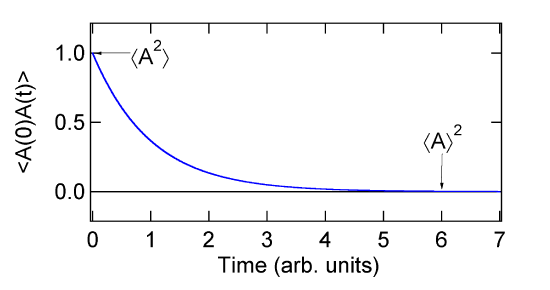
The decay shown in the figure is the average of the decay in many ensembles (time origins if we are using the output from a MD simulation). The decay in any single ensemble would be very noisy. We can see that \(C(t)\) decays from \(\langle A^2\rangle \) to \(\langle A\rangle^2 \).

\[\langle A^2\rangle \ge C(t) \ge \langle A\rangle^2 \]

Spectral Density

The spectral density is the Fourier transform of the correlation function. The most direct route to understanding this definition is the time-correlation function for the absorption or emission of a photon. The time-dependent Schrödinger equation is

\[ H \Psi = i\hbar \dfrac{\partial}{\partial t} \Psi\]

The formal solution is

\[ \Psi(t) = e^{-i Ht/\hbar} \Psi = e^{-i Et/\hbar} \Psi\]

where the following definitions apply

We can treat an applied electromagnetic field as a perturbation to the Hamiltonian. The zeroth order Hamiltonian (that of system without the field) is H₀. The field Hamiltonian is \(- \mu \cdot E\). The total Hamiltonian is

\[ H = H_o + H_1= H_o - \mu \cdot E\]

We consider two states, an initial state i and a final state f. The transition probability between the two states is

This expression is an approximate solution known as the Fermi golden rule. Omitting a number of steps we can define the intensity of absorbed or emitted radiation as

where

\[p_i = \exp \left( \dfrac{-\hbar \omega_i}{kT}\right)\]

The delta function in the Golden Rule and intensity expressions can be represented by the integral

\[\delta (\omega) = \int_{-\infty}^{\infty} e^{-i \omega t} dt\]

Using the Einstein relation

\[ \omega_{fi} = \dfrac{E_f-E_i}{\hbar}\]

the delta function in the intensity expression is

We can replace the delta function in the intensity expression with the above integral and apply

as an operator

The time dependent dipole operator is defined in Heisenberg representation where a time-dependent operator is related to a static operator by

\[ A(t) = e^{i H t/\hbar}A(0)e^{-i H t/\hbar} \]

The above transformation is valid if \(|i \rangle\) and \(|f \rangle\) are eigenfunctions of the same Hamiltonian. This is the case for vibrational and rotational transitions, but not electronic transitions. Using the above formalism the intensity is

The individual matrix elements \(\langle i| \mu |f\rangle\) are just numbers so the order of multiplication does not matter. Since the final states form a complete set we can use the closure relation

\[ \sum_f | f \rangle \langle f | = 1\]

This results in

The sum over initial states is a weighted Boltzmann average (pi is the Boltzmann weighting factor) so this is nothing more than an ensemble average. Thus, we can write

Since this represents the ensemble averaged dipole moment, m here really represents the system dipole moment. For example, ám(0)m(¥)ñ = 0 since the isotropically averaged dipole moment points in all directions of space with equal probability and cancels.

Since we have considered the intensity of absorbed radiation we can use the following definitions for m to relate explicitly to spectra.

Microwave or far infrared: \(\mu = \mu_o\), the permanent dipole moment of the molecule.
Infrared: \(\mu = (\partial \mu /\partial Q)Q\) where \(Q\) is a normal coordinate of vibration
Rayleigh scattering: \(\mu = \mu_{ind} µ eI_ \cdot \alpha \cdot e_s \) where \(\alpha\) is the ground state polarizability and e_i and e_s are the direction of incident and scattered radiation, respectively.
Raman scattering: \(\mu= \mu_{ind} \propt e_i \cdot(\partial \alpha /\partial Q) \cdot e_s\)

Example \(\PageIndex{1}\):

We can consider three important examples that can be used to calculate spectral line shapes

\(C(t) = C(0)\) then \(I = I_0 \delta (\omega - \omega_o )\)
C(t) = C(0)(1/Ö 2pt )exp(-t²/2t² ), I = I₀ exp(-w²t² /4)
C(t) = C(0)exp(-t/t ), I = t /(1 + w²t² )

Once substituted into the Fourier transform the integral is no longer a Gaussian integral. However, the function can be converted into a Gaussian by completing the square. We complete the square by adding a term in the exponent that depends only on frequency and hence is a constant with respect to the integration over time.