9: Diffusion
- Page ID
- 1392
\( \newcommand{\vecs}[1]{\overset { \scriptstyle \rightharpoonup} {\mathbf{#1}} } \)
\( \newcommand{\vecd}[1]{\overset{-\!-\!\rightharpoonup}{\vphantom{a}\smash {#1}}} \)
\( \newcommand{\dsum}{\displaystyle\sum\limits} \)
\( \newcommand{\dint}{\displaystyle\int\limits} \)
\( \newcommand{\dlim}{\displaystyle\lim\limits} \)
\( \newcommand{\id}{\mathrm{id}}\) \( \newcommand{\Span}{\mathrm{span}}\)
( \newcommand{\kernel}{\mathrm{null}\,}\) \( \newcommand{\range}{\mathrm{range}\,}\)
\( \newcommand{\RealPart}{\mathrm{Re}}\) \( \newcommand{\ImaginaryPart}{\mathrm{Im}}\)
\( \newcommand{\Argument}{\mathrm{Arg}}\) \( \newcommand{\norm}[1]{\| #1 \|}\)
\( \newcommand{\inner}[2]{\langle #1, #2 \rangle}\)
\( \newcommand{\Span}{\mathrm{span}}\)
\( \newcommand{\id}{\mathrm{id}}\)
\( \newcommand{\Span}{\mathrm{span}}\)
\( \newcommand{\kernel}{\mathrm{null}\,}\)
\( \newcommand{\range}{\mathrm{range}\,}\)
\( \newcommand{\RealPart}{\mathrm{Re}}\)
\( \newcommand{\ImaginaryPart}{\mathrm{Im}}\)
\( \newcommand{\Argument}{\mathrm{Arg}}\)
\( \newcommand{\norm}[1]{\| #1 \|}\)
\( \newcommand{\inner}[2]{\langle #1, #2 \rangle}\)
\( \newcommand{\Span}{\mathrm{span}}\) \( \newcommand{\AA}{\unicode[.8,0]{x212B}}\)
\( \newcommand{\vectorA}[1]{\vec{#1}} % arrow\)
\( \newcommand{\vectorAt}[1]{\vec{\text{#1}}} % arrow\)
\( \newcommand{\vectorB}[1]{\overset { \scriptstyle \rightharpoonup} {\mathbf{#1}} } \)
\( \newcommand{\vectorC}[1]{\textbf{#1}} \)
\( \newcommand{\vectorD}[1]{\overrightarrow{#1}} \)
\( \newcommand{\vectorDt}[1]{\overrightarrow{\text{#1}}} \)
\( \newcommand{\vectE}[1]{\overset{-\!-\!\rightharpoonup}{\vphantom{a}\smash{\mathbf {#1}}}} \)
\( \newcommand{\vecs}[1]{\overset { \scriptstyle \rightharpoonup} {\mathbf{#1}} } \)
\(\newcommand{\longvect}{\overrightarrow}\)
\( \newcommand{\vecd}[1]{\overset{-\!-\!\rightharpoonup}{\vphantom{a}\smash {#1}}} \)
\(\newcommand{\avec}{\mathbf a}\) \(\newcommand{\bvec}{\mathbf b}\) \(\newcommand{\cvec}{\mathbf c}\) \(\newcommand{\dvec}{\mathbf d}\) \(\newcommand{\dtil}{\widetilde{\mathbf d}}\) \(\newcommand{\evec}{\mathbf e}\) \(\newcommand{\fvec}{\mathbf f}\) \(\newcommand{\nvec}{\mathbf n}\) \(\newcommand{\pvec}{\mathbf p}\) \(\newcommand{\qvec}{\mathbf q}\) \(\newcommand{\svec}{\mathbf s}\) \(\newcommand{\tvec}{\mathbf t}\) \(\newcommand{\uvec}{\mathbf u}\) \(\newcommand{\vvec}{\mathbf v}\) \(\newcommand{\wvec}{\mathbf w}\) \(\newcommand{\xvec}{\mathbf x}\) \(\newcommand{\yvec}{\mathbf y}\) \(\newcommand{\zvec}{\mathbf z}\) \(\newcommand{\rvec}{\mathbf r}\) \(\newcommand{\mvec}{\mathbf m}\) \(\newcommand{\zerovec}{\mathbf 0}\) \(\newcommand{\onevec}{\mathbf 1}\) \(\newcommand{\real}{\mathbb R}\) \(\newcommand{\twovec}[2]{\left[\begin{array}{r}#1 \\ #2 \end{array}\right]}\) \(\newcommand{\ctwovec}[2]{\left[\begin{array}{c}#1 \\ #2 \end{array}\right]}\) \(\newcommand{\threevec}[3]{\left[\begin{array}{r}#1 \\ #2 \\ #3 \end{array}\right]}\) \(\newcommand{\cthreevec}[3]{\left[\begin{array}{c}#1 \\ #2 \\ #3 \end{array}\right]}\) \(\newcommand{\fourvec}[4]{\left[\begin{array}{r}#1 \\ #2 \\ #3 \\ #4 \end{array}\right]}\) \(\newcommand{\cfourvec}[4]{\left[\begin{array}{c}#1 \\ #2 \\ #3 \\ #4 \end{array}\right]}\) \(\newcommand{\fivevec}[5]{\left[\begin{array}{r}#1 \\ #2 \\ #3 \\ #4 \\ #5 \\ \end{array}\right]}\) \(\newcommand{\cfivevec}[5]{\left[\begin{array}{c}#1 \\ #2 \\ #3 \\ #4 \\ #5 \\ \end{array}\right]}\) \(\newcommand{\mattwo}[4]{\left[\begin{array}{rr}#1 \amp #2 \\ #3 \amp #4 \\ \end{array}\right]}\) \(\newcommand{\laspan}[1]{\text{Span}\{#1\}}\) \(\newcommand{\bcal}{\cal B}\) \(\newcommand{\ccal}{\cal C}\) \(\newcommand{\scal}{\cal S}\) \(\newcommand{\wcal}{\cal W}\) \(\newcommand{\ecal}{\cal E}\) \(\newcommand{\coords}[2]{\left\{#1\right\}_{#2}}\) \(\newcommand{\gray}[1]{\color{gray}{#1}}\) \(\newcommand{\lgray}[1]{\color{lightgray}{#1}}\) \(\newcommand{\rank}{\operatorname{rank}}\) \(\newcommand{\row}{\text{Row}}\) \(\newcommand{\col}{\text{Col}}\) \(\renewcommand{\row}{\text{Row}}\) \(\newcommand{\nul}{\text{Nul}}\) \(\newcommand{\var}{\text{Var}}\) \(\newcommand{\corr}{\text{corr}}\) \(\newcommand{\len}[1]{\left|#1\right|}\) \(\newcommand{\bbar}{\overline{\bvec}}\) \(\newcommand{\bhat}{\widehat{\bvec}}\) \(\newcommand{\bperp}{\bvec^\perp}\) \(\newcommand{\xhat}{\widehat{\xvec}}\) \(\newcommand{\vhat}{\widehat{\vvec}}\) \(\newcommand{\uhat}{\widehat{\uvec}}\) \(\newcommand{\what}{\widehat{\wvec}}\) \(\newcommand{\Sighat}{\widehat{\Sigma}}\) \(\newcommand{\lt}{<}\) \(\newcommand{\gt}{>}\) \(\newcommand{\amp}{&}\) \(\definecolor{fillinmathshade}{gray}{0.9}\)Diffusion can be described as the random movement of particles through space, usually due to a concentration gradient. Diffusion is a spontaneous process and is a result of the random thermal motions between two particles. The diffusion coefficient (\(D\)) can be solved for with Fick’s laws of diffusion, which are broken up into two laws.
Fick’s First Law of Diffusion
Fick's first law of diffusion is given by the following equation:
\[ J = -D \dfrac{dc}{dx} \label{1} \]
where
- \(J\) is the flux and is defined by the number or particles that are moving past a given region divided by the area of that region multiplied by the time interval.
- The units of \(J\) are mol m-2 s-1.
- The letter \(D\) represents the diffusion coefficient with units m2 s and
- \(c\) is the concentration of the gradient with units molecules m-3.
Equation \ref{1} indicates that if the flux and the change in the concentration over time are known, then the diffusion coefficient can be calculated. The negative sign indicates that the concentration gradient is negative. The first law can only be applied to systems in which the conditions remain the same— in other words, if the flux coming into the system equals the flux going out. Fick’s second law is more applicable to physical science and other systems that are changing. This second law is applied to systems in which the condition are not steady, or the solution in not equal throughout.
Fick’s Second Law of Diffusion
\[ \dfrac{dc}{dt} = D \dfrac{d^2c}{dx^2} \label{2} \]
Where \( \frac{dc}{dt} \) represents the rate of change of concentration in a certain area and \( \frac{d^2c}{dx^2} \) represents the changes that the change in concentration can take; this would not be a smooth curve. This term accounts for a varying concentration in the system. If the concentration does not vary, then
\[ \dfrac{d^2c}{dx^2} = 0 \label{3} \]
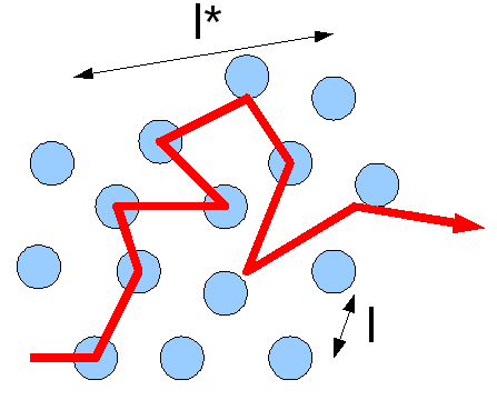
Diffusion can be thought of as a series of random steps that the particle takes as it moves from where it started. These steps can either lead the particle away from where it started, or lead back to where it started. This means that the overall path that a particle takes can look like line overlapping itself multiple times. A third way to calculate the diffusion concentration is through the Einstein-Smoluchowski equation:
\[ D = \dfrac{\lambda^2}{2\tau} \label{4} \]
where \(λ\) is the length that each step takes, and \(τ\) is the time that each step takes. In this particular model, each step is the same distance.

The diffusion coefficient is useful because it can tell you something about the system. For example, different substances have different diffusion coefficients, so knowing this can give you an idea of the substance. Ions at room temperature usually have a diffusion coefficient of 0.6×10⁻⁹ to 2×10⁻⁹ m2/s, and biological molecules fall in the range 10-11 to 10-10 m2/s. The diffusion coefficient changes as the properties of the system change. For example, at higher temperatures, the diffusion coefficient is greater because the molecules have more thermal motion. The diffusion coefficient is also related to the viscosity of the solution. The greater the diffusion coefficient, the lower the viscosity. Because the rate of diffusion depends on the temperature of the system, the Arrhenius equation can be applied. Applying this equation gives:
\[ D = [D]_{o}e^{-Ea/RT} \label{5} \]
The dependence of the diffusion coefficient on the viscosity can be modeled by the Stokes-Einstein relation:
\[ D = \dfrac{kT}{6\pi\eta{a}} \label{6} \]
where a is the radius of the molecule and η is the coefficient of viscosity and is defined by:
\[ \eta = \eta_o{e^{Ea/RT}} \label{7} \]
This equation demonstrates the dependence of viscosity on temperature.
Contributors and Attributions
- Laura Dickson (UC Davis)

