Stirling’s Approximation
- Page ID
- 2013
\( \newcommand{\vecs}[1]{\overset { \scriptstyle \rightharpoonup} {\mathbf{#1}} } \)
\( \newcommand{\vecd}[1]{\overset{-\!-\!\rightharpoonup}{\vphantom{a}\smash {#1}}} \)
\( \newcommand{\dsum}{\displaystyle\sum\limits} \)
\( \newcommand{\dint}{\displaystyle\int\limits} \)
\( \newcommand{\dlim}{\displaystyle\lim\limits} \)
\( \newcommand{\id}{\mathrm{id}}\) \( \newcommand{\Span}{\mathrm{span}}\)
( \newcommand{\kernel}{\mathrm{null}\,}\) \( \newcommand{\range}{\mathrm{range}\,}\)
\( \newcommand{\RealPart}{\mathrm{Re}}\) \( \newcommand{\ImaginaryPart}{\mathrm{Im}}\)
\( \newcommand{\Argument}{\mathrm{Arg}}\) \( \newcommand{\norm}[1]{\| #1 \|}\)
\( \newcommand{\inner}[2]{\langle #1, #2 \rangle}\)
\( \newcommand{\Span}{\mathrm{span}}\)
\( \newcommand{\id}{\mathrm{id}}\)
\( \newcommand{\Span}{\mathrm{span}}\)
\( \newcommand{\kernel}{\mathrm{null}\,}\)
\( \newcommand{\range}{\mathrm{range}\,}\)
\( \newcommand{\RealPart}{\mathrm{Re}}\)
\( \newcommand{\ImaginaryPart}{\mathrm{Im}}\)
\( \newcommand{\Argument}{\mathrm{Arg}}\)
\( \newcommand{\norm}[1]{\| #1 \|}\)
\( \newcommand{\inner}[2]{\langle #1, #2 \rangle}\)
\( \newcommand{\Span}{\mathrm{span}}\) \( \newcommand{\AA}{\unicode[.8,0]{x212B}}\)
\( \newcommand{\vectorA}[1]{\vec{#1}} % arrow\)
\( \newcommand{\vectorAt}[1]{\vec{\text{#1}}} % arrow\)
\( \newcommand{\vectorB}[1]{\overset { \scriptstyle \rightharpoonup} {\mathbf{#1}} } \)
\( \newcommand{\vectorC}[1]{\textbf{#1}} \)
\( \newcommand{\vectorD}[1]{\overrightarrow{#1}} \)
\( \newcommand{\vectorDt}[1]{\overrightarrow{\text{#1}}} \)
\( \newcommand{\vectE}[1]{\overset{-\!-\!\rightharpoonup}{\vphantom{a}\smash{\mathbf {#1}}}} \)
\( \newcommand{\vecs}[1]{\overset { \scriptstyle \rightharpoonup} {\mathbf{#1}} } \)
\(\newcommand{\longvect}{\overrightarrow}\)
\( \newcommand{\vecd}[1]{\overset{-\!-\!\rightharpoonup}{\vphantom{a}\smash {#1}}} \)
\(\newcommand{\avec}{\mathbf a}\) \(\newcommand{\bvec}{\mathbf b}\) \(\newcommand{\cvec}{\mathbf c}\) \(\newcommand{\dvec}{\mathbf d}\) \(\newcommand{\dtil}{\widetilde{\mathbf d}}\) \(\newcommand{\evec}{\mathbf e}\) \(\newcommand{\fvec}{\mathbf f}\) \(\newcommand{\nvec}{\mathbf n}\) \(\newcommand{\pvec}{\mathbf p}\) \(\newcommand{\qvec}{\mathbf q}\) \(\newcommand{\svec}{\mathbf s}\) \(\newcommand{\tvec}{\mathbf t}\) \(\newcommand{\uvec}{\mathbf u}\) \(\newcommand{\vvec}{\mathbf v}\) \(\newcommand{\wvec}{\mathbf w}\) \(\newcommand{\xvec}{\mathbf x}\) \(\newcommand{\yvec}{\mathbf y}\) \(\newcommand{\zvec}{\mathbf z}\) \(\newcommand{\rvec}{\mathbf r}\) \(\newcommand{\mvec}{\mathbf m}\) \(\newcommand{\zerovec}{\mathbf 0}\) \(\newcommand{\onevec}{\mathbf 1}\) \(\newcommand{\real}{\mathbb R}\) \(\newcommand{\twovec}[2]{\left[\begin{array}{r}#1 \\ #2 \end{array}\right]}\) \(\newcommand{\ctwovec}[2]{\left[\begin{array}{c}#1 \\ #2 \end{array}\right]}\) \(\newcommand{\threevec}[3]{\left[\begin{array}{r}#1 \\ #2 \\ #3 \end{array}\right]}\) \(\newcommand{\cthreevec}[3]{\left[\begin{array}{c}#1 \\ #2 \\ #3 \end{array}\right]}\) \(\newcommand{\fourvec}[4]{\left[\begin{array}{r}#1 \\ #2 \\ #3 \\ #4 \end{array}\right]}\) \(\newcommand{\cfourvec}[4]{\left[\begin{array}{c}#1 \\ #2 \\ #3 \\ #4 \end{array}\right]}\) \(\newcommand{\fivevec}[5]{\left[\begin{array}{r}#1 \\ #2 \\ #3 \\ #4 \\ #5 \\ \end{array}\right]}\) \(\newcommand{\cfivevec}[5]{\left[\begin{array}{c}#1 \\ #2 \\ #3 \\ #4 \\ #5 \\ \end{array}\right]}\) \(\newcommand{\mattwo}[4]{\left[\begin{array}{rr}#1 \amp #2 \\ #3 \amp #4 \\ \end{array}\right]}\) \(\newcommand{\laspan}[1]{\text{Span}\{#1\}}\) \(\newcommand{\bcal}{\cal B}\) \(\newcommand{\ccal}{\cal C}\) \(\newcommand{\scal}{\cal S}\) \(\newcommand{\wcal}{\cal W}\) \(\newcommand{\ecal}{\cal E}\) \(\newcommand{\coords}[2]{\left\{#1\right\}_{#2}}\) \(\newcommand{\gray}[1]{\color{gray}{#1}}\) \(\newcommand{\lgray}[1]{\color{lightgray}{#1}}\) \(\newcommand{\rank}{\operatorname{rank}}\) \(\newcommand{\row}{\text{Row}}\) \(\newcommand{\col}{\text{Col}}\) \(\renewcommand{\row}{\text{Row}}\) \(\newcommand{\nul}{\text{Nul}}\) \(\newcommand{\var}{\text{Var}}\) \(\newcommand{\corr}{\text{corr}}\) \(\newcommand{\len}[1]{\left|#1\right|}\) \(\newcommand{\bbar}{\overline{\bvec}}\) \(\newcommand{\bhat}{\widehat{\bvec}}\) \(\newcommand{\bperp}{\bvec^\perp}\) \(\newcommand{\xhat}{\widehat{\xvec}}\) \(\newcommand{\vhat}{\widehat{\vvec}}\) \(\newcommand{\uhat}{\widehat{\uvec}}\) \(\newcommand{\what}{\widehat{\wvec}}\) \(\newcommand{\Sighat}{\widehat{\Sigma}}\) \(\newcommand{\lt}{<}\) \(\newcommand{\gt}{>}\) \(\newcommand{\amp}{&}\) \(\definecolor{fillinmathshade}{gray}{0.9}\)Stirling's approximation is named after the Scottish mathematician James Stirling (1692-1770). In confronting statistical problems we often encounter factorials of very large numbers. The factorial \(N!\) is a product \(N(N-1)(N-2)...(2)(1)\). Therefore, \(\ln \,N!\) is a sum
\[\left.\ln N!\right. = \ln 1 + \ln 2 + \ln 3 + ... + \ln N = \sum_{k=1}^N \ln k. \label{1} \]
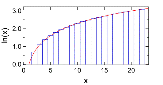
where we have used the property of logarithms that \(\log(abc) =\log(a) + \log(b) +\log(c)\). The sum is shown in figure below.

Using Euler-MacLaurin formula one has
\[\sum_{k=1}^N \ln k=\int_1^N \ln x\,dx+\sum_{k=1}^p\frac{B_{2k}}{2k(2k-1)}\left(\frac{1}{n^{2k-1}}-1\right)+R , \label{2} \]
where B1 = −1/2, B2 = 1/6, B3 = 0, B4 = −1/30, B5 = 0, B6 = 1/42, B7 = 0, B8 = −1/30, ... are the Bernoulli numbers, and \(R\) is an error term which is normally small for suitable values of \(p\).
Then, for large \(N\),
\[\ln N! \sim \int_1^N \ln x\,dx \approx N \ln N -N . \label{3} \]
after some further manipulation one arrives at (apparently Stirling's contribution was the prefactor of \(\sqrt{2\pi})\)
\[N! = \sqrt{2 \pi N} \; N^{N} e^{-N} e^{\lambda_N} \label{4} \]
where
\[\dfrac{1}{12N+1} < \lambda_N < \frac{1}{12N}. \label{5} \]
The sum of the area under the blue rectangles shown below up to \(N\) is \(\ln N!\). As you can see the rectangles begin to closely approximate the red curve as \(m\) gets larger. The area under the curve is given the integral of \(\ln x\).
\[ \ln N! = \sum_{m=1}^N \ln m \approx \int_1^N \ln x\, dx \label{6} \]
To solve the integral use integration by parts
\[ \int u\,dv=uv-\int v\,dy \label{7A} \]
Here we let \(u = \ln x\) and \(dv = dx\). Then \(v = x\) and \(du = \frac{dx}{x}\).
\[ \int_0^N \ln x \, dx = x \ln x|_0^N - \int_0^N x \dfrac{dx}{x} \label{7B} \]
Notice that \(x/x = 1\) in the last integral and \(x \ln x\) is 0 when evaluated at zero, so we have
\[ \int_0^N \ln x \, dx = N \ln N - \int_0^N dx \label{8} \]
Which gives us Stirling’s approximation: \(\ln N! = N \ln N – N\). As is clear from the figure above Stirling’s approximation gets better as the number N gets larger (Table \(\PageIndex{1}\)).
| N | N! | ln N! | N ln N – N | Error |
|---|---|---|---|---|
| 10 | 3.63 x 10⁶ | 15.1 | 13.02 | 13.8% |
| 50 | 3.04 x 1064 | 148.4 | 145.6 | 1.88% |
| 100 | 9.33 x 10157 | 363.7 | 360.5 | 0.88% |
| 150 | 5.71 x 10262 | 605.0 | 601.6 | 0.56% |
Calculators often overheat at 200!, which is all right since clearly result are converging. In thermodynamics, we are often dealing very large N (i.e., of the order of Avagadro’s number) and for these values Stirling’s approximation is excellent.
References
- J. Stirling "Methodus differentialis, sive tractatus de summation et interpolation serierum infinitarium", London (1730). English translation by J. Holliday "The Differential Method: A Treatise of the Summation and Interpolation of Infinite Series" (1749)

