4.2: Associative Ligand Substitution

Despite the sanctity of the 18-electron rule to many students of organometallic chemistry, a wide variety of stable complexes possess fewer than 18 total electrons at the metal center. Perhaps the most famous examples of these complexes are 14- and 16-electron complexes of group 10 metals involved in cross-coupling reactions.

Ligand substitution in complexes of this class typically occurs via an associative mechanism, involving approach of the incoming ligand to the complex before departure of the leaving group. If we keep this principle in mind, it seems easy enough to predict when ligand substitution is likely to be associative. But how can we spot an associative mechanism in experimental data, and what are some of the consequences of this mechanism?

The prototypical mechanism of associative ligand substitution. The first step is rate-determining. A typical mechanism for associative ligand substitution is shown above. It should be noted that square pyramidal geometry is also possible for the intermediate, but is less common. Let’s begin with the kinetics of the reaction.

Reaction Kinetics

Reaction kinetics are commonly used to elucidate organometallic reaction mechanisms, and ligand substitution is no exception. Different mechanisms of substitution may follow different rate laws, so plotting the dependence of reaction rate on concentration often allows us to distinguish mechanisms. Associative substitution’s rate law is analogous to that of the S_N2 reaction—rate depends on the concentrations of both starting materials.

\[ L_nM–L^d + L_i → L_nM–L_i + L^d \]

\[ \dfrac{d[L_nM–L^i]}{dt} = rate = k_1[L_nM–L^d][L^i] \]

The easiest way to determine this rate law is to use pseudo-first-order conditions. Although the rate law is second order overall, if we could somehow render the concentration of the incoming ligand unchanging, the reaction would appear first order. The observed rate constant under these conditions reflects the constancy of the incoming ligand’s concentration (\(k_{obs} = k_1[L^i]\), where both \(k_1\) and \([Li]\) are constants). How can we make the concentration of the incoming ligand invariant, you ask? We can drown the reaction in ligand to achieve this. The teensy weensy bit actually used up in the reaction has a negligible effect on the concentration of the “sea” of starting ligand we began with. The observed rate is equal to \(k_{obs}[L_nM–L^d]\), as shown by the purple trace below. By determining \(k_{obs}\) at a variety of \([L^i]\) values, we can finally isolate \(k_1\), the rate constant for the slow step. The red trace below at right shows the idea.

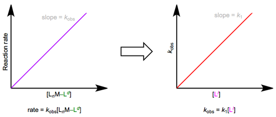
Associative substitution under pseudo-first-order conditions. The reaction is “swamped out” with incoming ligand.

In many cases, the red trace ends up with a non-zero y-intercept…curious, if we limit ourselves to the simple mechanism shown in the first figure of this post. A non-zero intercept suggests a more complex mechanism. We need to add a new term (called \(k_s\) for reasons to become clear shortly) to our first set of equations:

\[rate = (k_1[L_i] + k_s)[L_nM–L^d]\]

\[k_{obs} = k_1[L_i] + k_s\]

The full rate law suggests that some other step (with rate ks[LnM–Ld]) independent of incoming ligand is involved in the mechanism. To explain this observation, we can invoke the solvent as a reactant. Solvent can associate with the complex first in a slow step, then incoming ligand can displace the solvent in a fast step. Solvent concentration doesn’t enter the rate law because, well, it’s drowning the reactants and its concentration undergoes negligible change! An example of this mechanism in the context of Pt(II) chemistry is shown below.

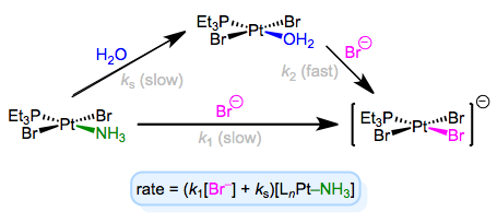
Associative substitution with solvent participation—a head-scratching mechanism for many an organometallic grad student!

As an aside, it’s worth mentioning that the entropy of activation of associative substitution is typically negative. Entropy decreases as the incoming ligand and complex come together in the rate-determining step. Dissociative substitution shows the opposite behavior: loss of the departing ligand in the RDS increases entropy, resulting in positive entropy of activation.

Stereochemistry of Substitution

As we saw in discussions of the trans effect, the entering and departing ligands both occupy equatorial positions in the trigonal bipyramidal intermediate. Microscopic reversibility is to blame: the mechanism of the forward substitution (displacement of the leaving by the incoming ligand) must be the same as the mechanism of the reverse reaction (displacement of the incoming by the leaving ligand). This can be a confusing point, so let’s examine an alternative mechanism that violates microscopic reversibility.

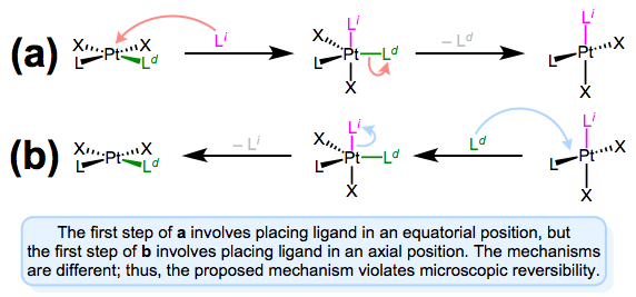
A mechanism involving approach to an axial position and departure from an equatorial position violates microscopic reversibility. Forward and reverse reactions a and b differ!

The figure above shows why a mechanism involving axial approach and equatorial departure (or vice versa) is not possible. The forward and reverse reactions differ, in fact, in both steps. In forward mechanism a, the incoming ligand enters an axial site. But in the reverse reaction, the incoming ligand (viz., the departing ligand in mechanism a) sits on an equatorial site. The second steps of each mechanism differ too—a involves loss of an equatorial ligand, while b involves loss of an axial ligand. Long story short, this mechanism violates microscopic reversibility. And what about a mechanism involving axial approach and axial departure? Such a mechanism is unlikely on electronic grounds. The equatorial sites are more electron rich than the axial sites, and σ bonding to the axial \(d_{z^2}\) orbital is expected to be strong. Intuitively, then, loss of ligand from an axial site is less favorable than loss from an equatorial site.

I know what you’re thinking: what the heck does all of this have to do with stereochemistry? Notice that, in the equatorial-equatorial mechanism (first figure of this post), the axial ligands don’t move at all. The configuration of the starting complex is thus retained in the product. Although retention is “normal,” complications often arise because five-coordinate TBP complexes—like other odd-coordinate organometallic complexes—are often fluxional. Axial and equatorial ligands can rapidly exchange through a process called Berry pseudorotation, which resembles the axial ligands “cutting through” a pair of equatorial ligands like scissors (animation!). Fluxionality means that all stereochemical bets are off, since any ligand can feasibly occupy an equatorial site. In the example below, the departing ligand starts out cis to L, but the incoming ligand ends up trans to L.

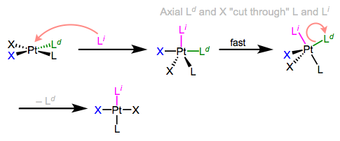
Berry pseudorotation in the midst of associative ligand substitution.

Associative Substitution in 18-electron Complexes?

Associative substitution can occur in 18-electron complexes if it’s preceded by the dissociation of a ligand. For example, changes in the hapticity of cyclopentadienyl or indenyl ligands may open up a coordination site, which can be occupied by a new ligand to kick off associative substitution. An allyl ligand may convert from its π to σ form, leaving an open coordination site where the π bond left. A particularly interesting case is the nitrosyl ligand—conversion from its linear to bent form opens up a site for coordination of an external ligand.

Summary

Associative ligand substitution is common for complexes with 16 total electrons or fewer. The reaction is characterized by a second-order rate law, the possibility of solvent participation, and a trigonal bipyramidal intermediate that is often fluxional. An open coordination site is essential for associative substitution, but such sites are often hidden in the dynamism of 18-electron complexes with labile ligands.

Dr. Michael Evans (Georgia Tech)