15.3: Excitons in Molecular Aggregates

The absorption spectra of periodic arrays of interacting molecular chromophores show unique spectral features that depend on the size of the system and disorder of the environment. We will investigate some of these features, focusing on the delocalized eigenstates of these coupled chromophores, known as excitons. These principles apply to the study of molecular crystals, J-aggregates, photosensitizers, and light-harvesting complexes in photosynthesis. Similar topics are used in the description of properties of conjugated polymers and organic photovoltaics, and for extended vibrational states in IR and Raman spectroscopy.

Energy Transfer in the Strong Coupling Limit

Strong coupling between molecules leads to the delocalization of electronic or vibrational eigenstates, under which weak coupling models like FRET do not apply. From our studies of the coupled two-state system, we know that when the coupling between states is much larger that the energy splitting between the states (\(\varepsilon _ {1} - \varepsilon _ {2} \ll 2 \mathrm {V}\)) then the resulting eigenstates \(| \pm \rangle\) are equally weighted symmetric and antisymmetric combinations of the two, whose energy eigenvalues are split by \(2V\). Setting \(\varepsilon _ {1} = \varepsilon _ {2} = \varepsilon\)

\[E _ {\pm} = \varepsilon \pm V\]

\[| \pm \rangle = \frac {1} {\sqrt {2}} ( | 1 \rangle \pm | 2 \rangle )\]

If we excite one of these molecules, we expect that the excitation will flow back and forth at the Rabi frequency. So, what happens with multiple coupled chromophores, focusing particular interest on the placement of coupled chromophores into periodic arrays in space? In the strong coupling regime, the variation in the uncoupled energies is small, making this a problem of coupled quasi-degenerate states. With a spatially period structure, the resulting states bear close similarity to simple descriptions of electronic band structure using the tight-binding model.

Excitons

Excitons refer to electronic excited states that are not localized to a particular molecule. But beyond that there are many flavors. We will concentrate on Frenkel excitons, which refer to excited states in which the excited electron and the corresponding hole (or electron vacancy) reside on the same molecule. All molecules remain electrically neutral in the ground and excited states. This corresponds to what one would expect when one has resonant dipole–dipole interactions between molecules. When there is charge transfer character, the electron and hole can reside on different molecules of the coupled complex. These are referred to as Mott–Wannier excitons.

Absorption Spectrum of Molecular Dimer

To describe the spectroscopy of an array of many coupled chromophores, it is first instructive to work through a pair of coupled molecules. This is in essence the two-level problem from earlier. We consider a pair of molecules (\(1\) and \(2\)), which each have a ground and electronically excited state \(| e \rangle\) and \(| g \rangle\)) split by an energy gap \(\varepsilon 0\), and a transition dipole moment \(\overline {\mu}\). In the absence of coupling, the state of the system can be specified by specifying the electronic state of both molecules, leading to four possible states: \(|g g\rangle,|e g\rangle,|g e\rangle,|e e\rangle\) whose energies are \(0, \varepsilon_{0,} \varepsilon_{0}\), and \(2 \varepsilon 0\), respectively.

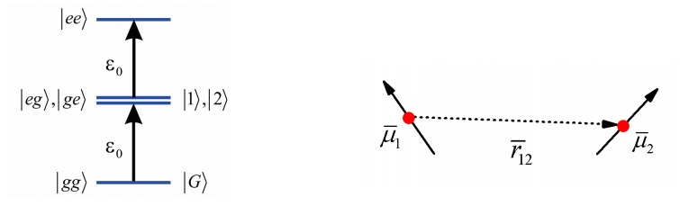
For shorthand we define the ground state as \(|G\rangle\) and the excited states as \(|1\rangle\) and \(|2\rangle\) to signify the the electronic excitation is on either molecule \(1\) or \(2\). In addition, the molecules are spaced by a separation \(r_{12}\), and there is a transition dipole interaction that couples the molecules.

\[V = J ( | 2 \rangle \langle 1 | + | 1 \rangle \langle 2 | )\]

Following our description of transition dipole coupling the coupling strength \(J\) is given by

\[J=\frac{\left(\bar{\mu}_{1} \cdot \bar{\mu}_{2}\right)\left|\bar{r}_{12}\right|^{2}-3\left(\bar{\mu}_{1} \cdot \bar{r}_{12}\right)\left(\bar{\mu}_{2} \cdot \bar{r}_{12}\right)}{\left|\bar{r}_{12}\right|^{5}}=\frac{\mu_{1} \mu_{2}}{r_{12}^{3}} \kappa\]

where the orientational factor is

\[\kappa=\left(\hat{\mu}_{1} \cdot \hat{\mu}_{2}\right)-3\left(\hat{\mu}_{1} \cdot \hat{r}_{12}\right)\left(\hat{\mu}_{2} \cdot \hat{r}_{12}\right)\]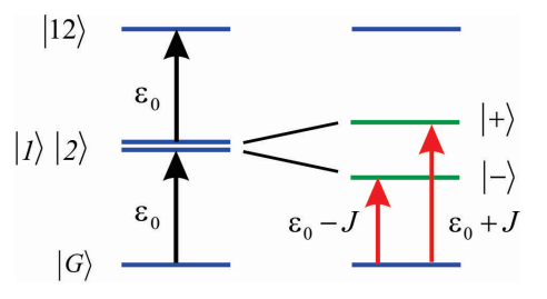

We assume that the coupling is not too strong, so that we can just concentrate on how it influences \(|1 \rangle\) and \(|2 \rangle\) but not \(|G \rangle\). Then we only need to describe the coupling induced shifts to the singly excited states, which are described by the Hamiltonian

\[H = \left( \begin{array} {l l} {\varepsilon _ {0}} & {J} \\ {J} & {\varepsilon _ {0}} \end{array} \right)\]

As stated above, we find that the eigenvalues are

\[E _ {\pm} = \varepsilon _ {0} \pm J\]

and that the eigenstates are:

\[|\pm\rangle=\frac{1}{\sqrt{2}}(|1\rangle \pm|2\rangle)\]

These symmetric and antisymmetric states are delocalized across the two molecules, and in the language of Frenkel excitons are referred to as the one-exciton states. Furthermore, the dipole operator for the dimer is

\[\overline {M} = \overline {\mu} _ {1} + \overline {\mu} _ {2}\]

and so the transition dipole matrix elements are:

\[M _ {\pm} = \langle \pm | \overline {M} | G \rangle = \frac {1} {\sqrt {2}} \left( \overline {\mu} _ {1} \pm \overline {\mu} _ {2} \right)\]

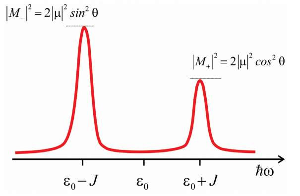
\(M_+\) and \(M_-\) are oriented perpendicular to each other in the molecular frame. If we confine the molecular dipoles to be within a plane, with an angle \(2 \theta\) between them, then the amplitude of M+ and M- is given by

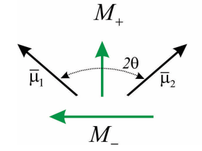
\begin{array}{l}
M_{+}=2 \mu \cos \theta \\
M_{-}=2 \mu \sin \theta
\end{array}

We can now predict the absorption spectrum for the dimer. We have two transitions from the ground state and the \(| \pm \rangle\) states which are resonant at \(\hbar \omega = \varepsilon _ {0} \pm J\) and which have an amplitude \(\left| M _ {*} \right|^{2}\). The splitting between the peaks is referred to as the Davydov splitting. Note that the relative amplitude of the peaks allows one to infer the angle between the molecular transition dipoles. Also, note for \(θ = 0°\) or \(90°\), all amplitude appears in one transition with magnitude \(2 | \mu |^{2}\), which is referred to as superradiant.

Frenkel Excitons with Periodic Boundary Conditions

Now let’s consider linear aggregate of \(N\) periodically arranged molecules. We will assume that each molecule is a two-level electronic system with a ground state and an excited state. We will assume that electronic excitation moves an electron from the ground state to an unoccupied orbital of the same molecule. We will label the molecules with integer values (\(n\)) between \(0\) and \(N-1\):

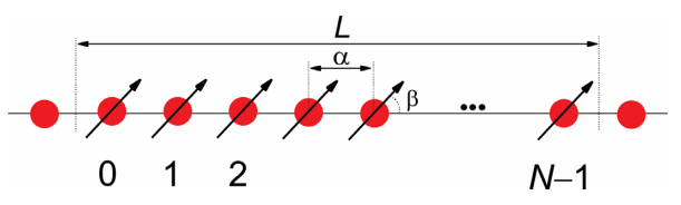
If the molecules are separated along the chain by a lattice spacing \(a\), then the size of the chain is \(L = \alpha N\). Each molecule has a transition dipole moment \(\mu\), which makes an angle \(\beta\) with the axis of the chain.

In the absence of interactions, we can specify the state of the system exactly by identifying whether each molecule is in the electronically excited or ground state. If the state of molecule n within the chain is \(\varphi _ {n}\), which can take on values of \(g\) or \(e\), then

\[| \psi \rangle = | \varphi _ {0} , \varphi _ {1} , \varphi _ {2} \cdots \varphi _ {n} \cdots \varphi _ {N - 1} \rangle\]

This representation of the state of the system is referred to as the site basis, since it is expressed in terms of each molecular site in the chain. For simplicity we write the ground state of the system as

\[| G \rangle = | g , g , g \ldots , g \rangle\]

If we excite one of the molecules within the aggregate, we have a singly excited state in which the nth molecule is excited, so that

\[| \psi \rangle = | g , g , g , \ldots , e , \dots , g \rangle \equiv | n \rangle\]

For shorthand, we identify this product state as \(| n \rangle\) which is to be distinguished from the molecular eigenfunction at site \(n\), \(\varphi _ {n}\).

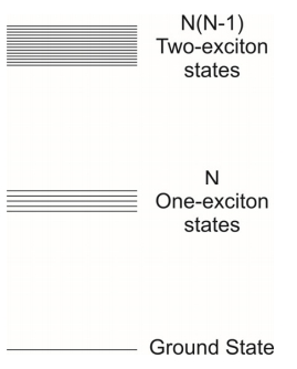
The singly excited state is assigned an energy \(\mathcal {E} _ {0}\) corresponding to the electronic energy gap. In the absence of coupling, the singly excited states are \(N\)-fold degenerate, corresponding to a single excitation at any of the \(N\) sites. If two excitations are placed on the chain we can see that there are \(N(N-1)\) possible states with energy \(2 \varepsilon _ {0}\), recognizing that the Pauli principle does not allow two excitations on the same site. When coupling is introduced, the mixing of these degenerate states leads to the one-exciton and two-exciton bands. For this discussion, we will concentrate on the one-exciton states.

The coupling between molecule \(n\) and molecule \(n′\) is given by the matrix element \(V _ {n n^{\prime}}\). We will assume that a molecule interacts only with its neighbors, and that each pairwise interaction has a magnitude \(J\)

\[V _ {n n^{\prime}} = J \delta _ {n , n^{\prime} \pm 1}\]

If \(V\) is a dipole–dipole interaction, the orientational factor \(\kappa\) dictates that when the transition dipole angle \(\beta < 54.7^{\circ}\) then the sign of the coupling \(J < 0\), which is the case known as J-aggregates (after Edwin Jelley), and implies an offset stack of chromophores or head-to-tail arrangement. If \(\beta > 54.7^{\circ}\) then \(J > 0\), and the system is known as an H-aggregate.

To begin, we also apply periodic boundary conditions to this problem, which implies that we are describing the states of an N-molecule chain within an infinite linear chain. In terms of the Hamiltonian, the molecules at the beginning and end of our chain feel the same symmetric interactions to two neighbors as the other molecules. To write this in terms of a finite \(N \times N\) matrix, one couples the first and last member of the chain: \(J _ {0 , N - 1} = J _ {N - 1,0} = J\)

\[J _ {0 , N - 1} = J _ {N - 1,0} = J.\]

With these observations in mind, we can write the Frenkel Exciton Hamiltonian for the linear aggregate in terms of a system Hamiltonian that reflects the individual sites and their couplings

\[\begin{align} H _ {0} &= H _ {S} + V \\[4pt] H _ {S} &= \sum _ {n = 1}^{N} \varepsilon _ {0} | n \rangle \langle n | \\[4pt] V &= \sum _ {n = 1}^{N} J \{| n^{\prime} \rangle \langle n | + | n \rangle \left\langle n^{\prime} | \right\} \delta _ {n , n^{\prime} \pm 1} \label{14.30} \end{align}\]

Here periodic boundary conditions imply that we replace \(| N \rangle \Rightarrow | 0 \rangle\) and \(| - 1 \rangle \Rightarrow | N - 1 \rangle\) where they appear.

The optical properties of the aggregate will be obtained by determining the eigenstates of the Hamiltonian. We look for solutions that describe one-exciton eigenstates as an expansion in the site basis.

\[| \psi (x) \rangle = \sum _ {n = 0}^{N - 1} c _ {n} ( \mathrm {x} ) | \varphi _ {n} \left( x - x _ {n} \right) \rangle \label{14.31}\]

which is written in order to point out the dependence of these wavefunctions on the lattice spacing x, and the position of a particular molecule at xn. Such an expansion should work well when the electronic interactions between sites is weak enough to treat perturbatively. For the electronic structure of solids, this is known as the tight binding model, which describes band structure as a linear combinations of atomic orbitals.

Rather than diagonalizing the Hamiltonian, we can take advantage of its translational symmetry to obtain the eigenstates. The symmetry of the Hamiltonian is such that it is unchanged by any integral number of translations along the chain. That is the results are unchanged for any summation in Equation \ref{14.30} and \ref{14.31} over \(N\) consecutive integers. Similarly, the molecular wavefunction at any site is unchanged by such a translation. Written in terms of a displacement operator \(D = e^{i p _ {x} \alpha / \hbar}\) that shifts the molecular wavefunction by one lattice constant

\[| \varphi ( x + n \alpha ) \rangle = D^{n} | \varphi (x) \rangle \label{14.32}\]

These observations underlie Bloch’s theorem, which states that the eigenstates of a periodic system will vary only by a phase shift when displaced by a lattice constant.

\[| \psi ( x + \alpha ) \rangle = e^{i k \alpha} | \psi (x) \rangle \label{14.33}\]

Here \(k\) is the wavevector, or reciprocal lattice vector, a real quantity. Thus the expansion coefficients in Equation \ref{14.31} will have an amplitude that reflects an excitation spread equally among the N sites, and only vary between sites by a spatially varying phase factor. Equivalently, the eigenstates are expected to have a form that is a product of a spatially varying phase factor and a periodic function:

\[| \psi (x) \rangle = e^{i k x} u (x) \label{14.34}\]

These phase factors are closely related to the lattice displacement operators. If the linear chain has \(N\) molecules, the eigenstates must remain unchanged with a translation by the length of the chain \(L = \alpha N\):

\[| \psi \left( x _ {n} + L \right) \rangle = | \psi \left( x _ {n} \right) \rangle\]

Therefore, we see that our wavefunctions must satisfy

\[ N k \alpha = 2 \pi m\label{14.35}\]

where \(m\) is an integer. Furthermore, since there are \(N\) sites on the chain, unique solutions to Equation \ref{14.35} require that \(m\) can only take on \(N\) consecutive integer values. Like the site index \(n\), there is no unique choice of \(m\). Rewriting Equation \ref{14.35}, the wavevector is

\[k _ {m} = \frac {2 \pi} {\alpha} \frac {m} {N} \label{14.36}\]

We see that for an \(N\) site lattice, \(m\) can take on the \(N\) consecutive integer values, so that \(k_m\alpha\) varies over a \(2\pi\) range of angles. The wavevector index m labels the \(N\) one-exciton eigenstates of an \(N\) molecule chain. By convention, \(k_m\) is chosen such that

\[- \pi / \alpha < k _ {m} \leq \pi / \alpha.\]

Then the corresponding values of \(m\) are integers from \(-N-1)/2\) to \(N-1/2\) if there are an odd number of lattice sites or \(-N-2)/2\) to \(N/2\) for an even number of sites. For example, a 20 molecule chain would have \(m = -9,\, -8,\, … 9,\,10\).

These findings lead to the general form for the m one-exciton eigenstates

\[| k _ {m} \rangle = \frac {1} {\sqrt {N}} \sum _ {n = 0}^{N - 1} e^{i n k _ {m} \alpha} | n \rangle \label{14.37}\]

The factor of \(\sqrt{N}\) assures proper normalization of the wavefunction, \(\langle \psi | \psi \rangle = 1\). Comparing Equation \ref{14.37} and \ref{14.31} we see that the expansion coefficients for the nth site of the mth eigenstate is

\[c _ {m , n} = \frac {1} {\sqrt {N}} e^{i n k _ {m} \alpha} = \frac {1} {\sqrt {N}} e^{i 2 \pi n m / N} \label{14.38}\]

We see that for state \(| k _ {0} \rangle\), with \(m = 0\), the phase factor is the same for all sites. In other words, the transition dipoles of the chain will oscillate in-phase, constructively adding for all sites. For the case that \(k _ {m} = \pi / \alpha\), we see that each site is out-of-phase with its nearest neighbors. Looking at the case of the dimer, \(N = 2\), we see that \(m = 0\) or \(1\), \(k_m = 0\) or \(\pi/2\), and we recover the expected symmetric and antisymmetric eigenstates:

\[| k _ {0} \rangle = \frac {1} {\sqrt {2}} \sum _ {n = 0}^{1} e^{i n 0} | n \rangle = \frac {1} {\sqrt {2}} ( | 0 \rangle + | 1 \rangle )\]

for \(k=0\) and

\[| k _ {1} \rangle = \frac {1} {\sqrt {2}} \sum _ {n = 0}^{1} e^{i n \pi} | n \rangle = \frac {1} {\sqrt {2}} ( | 0 \rangle - | 1 \rangle )\]

for \(k = \pi / \alpha\).

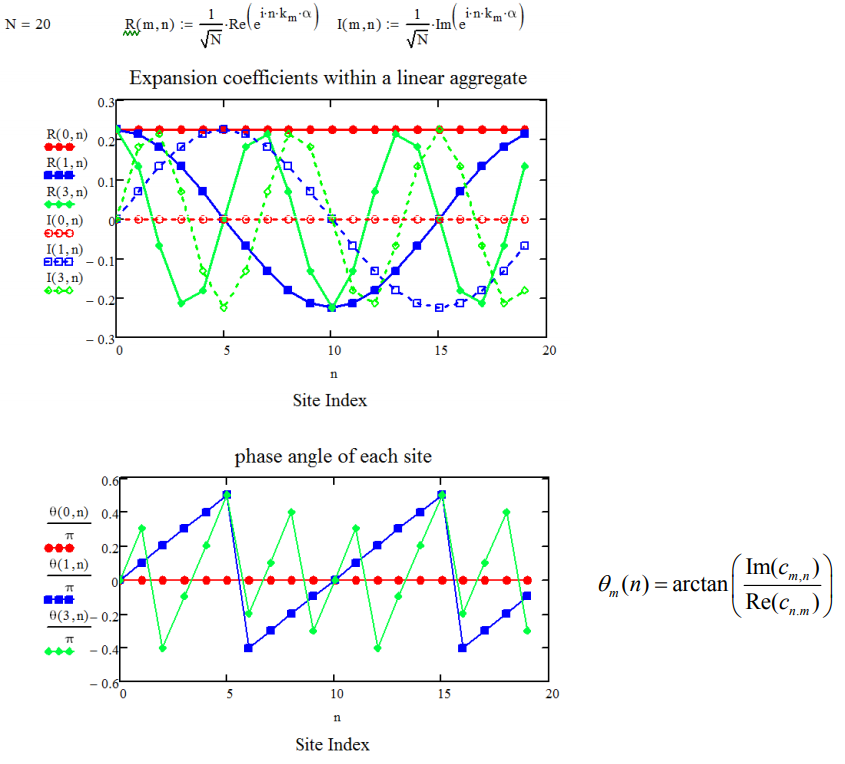
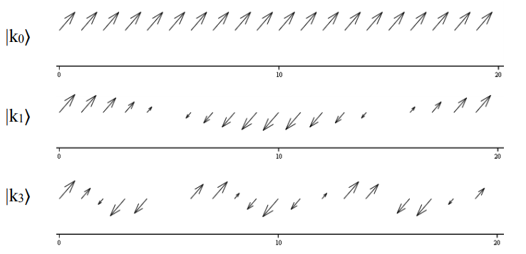
Schematically for \(N = 20\), we see how the dipole phase varies with \(k_m\), plotting the real and imaginary components of the expansion coefficients.

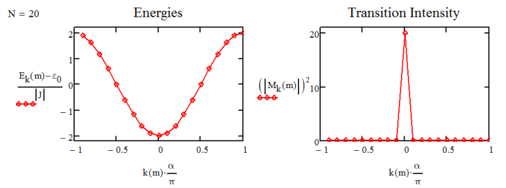
Also, we can evaluate the one-exciton transition dipole matrix elements, \(M(k_m)\), which are expressed as superpositions of the dipole moments at each site, \(\overline {\mu} _ {n}\):

\[\overline {M} = \sum _ {n = 0}^{N - 1} \overline {\mu} _ {n} \label{14.39}\]

\[\begin{align} M _ {m} = \left\langle k _ {m} | \overline {M} | G \right\rangle \\[4pt] = \frac {1} {\sqrt {N}} \sum _ {n = 0}^{N - 1} e^{i n k _ {n} \alpha} \left\langle n \left| \overline {\mu} _ {n} \right| G \right\rangle \label{14.40} \end{align}\]

The phase of the transition dipoles of the chain matches their phase within each k state. Thus for our problem, in which all of the dipoles are parallel, transitions from the ground state to the \(k_m=0\) state will carry all of the oscillator strength. Plotted below is an illustration of the phase relationships between dipoles in a chain with \(N = 20\).

Finally, let’s solve for the one-exciton energy eigenvalues by calculating the expectation value of the Hamiltonian operator, Equation \ref{14.30}

\[\begin{align} E \left( k _ {m} \right) &= \left\langle k \left| H _ {0} \right| k \right\rangle \\[4pt] &= \frac {1} {N} \sum _ {n , m = 0}^{N - 1} e^{i ( n - m ) k \alpha} \left\langle m \left| H _ {0} \right| n \right\rangle \label{14.41} \end{align} \]

\[\left\langle k _ {m} \left| H _ {S} \right| k _ {m} \right\rangle = \frac {1} {N} \sum _ {n = 0}^{N - 1} \varepsilon _ {0} = \varepsilon _ {0}\]

\[\begin{align} \left\langle k _ {m} | V | k _ {m} \right\rangle &= \frac {1} {N} \sum _ {n = 0}^{N - 1} \left\{e^{i k _ {m} \alpha} \langle n - 1 | V | n \rangle + e^{- i k _ {m} \alpha} \langle n + 1 | V | n \rangle \right\}\\[4pt] &= 2 J \cos \left( k _ {m} \alpha \right) \label{14.42} \end{align}\]

You predict that the one-exciton band of states varies in energy between \(\varepsilon _ {0} - 2 J\) and \(\varepsilon _ {0} + 2 J\). If we take J as negative, as expected for the case of J-aggregates (negative couplings), then \(k = 0\) is at the bottom of the band. Examples are illustrated below for the \(N=20\) aggregate.

Note that the result in Equation \ref{14.42} gives you a splitting of \(4J\) between the two states of the dimer, unlike the expected \(2J\) splitting from earlier. This is a result of the periodic boundary conditions that we enforce here. We are now in a position to plot the absorption spectrum for aggregate, summing over eigenstates and assuming a Lorentzian lineshape for the system:

\[\sigma ( \omega ) = \sum _ {m} \left| M _ {m} \right|^{2} \frac {\Gamma^{2}} {\left( \hbar \omega - E \left( k _ {m} \right) \right) + \Gamma^{2}}\]

For a 20 oscillator chain with negative coupling, the spectrum is plotted below. We have one peak corresponding to the k0 mode that is peaked at \(\hbar \omega = \varepsilon _ {0} - 2 J\) and carries the oscillator strength of all 20 dipoles.

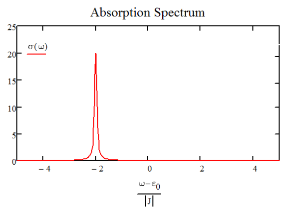
Absorption spectrum for \(N=20\) aggregate with periodic boundary conditions and \(J<0\).

Open Boundary Conditions

Similar types of solutions appear without using periodic boundary conditions. For the case of open boundary conditions, in the molecules at the end of the chain are only coupled to the one nearest neighbor in the chain. In this case, it is helpful to label on the sites from \(n = 1,2,...,N\). Furthermore, \(m = 1,2,...,N\). Under those conditions, one can solve for the eigenstates using use the boundary condition that \(\psi = 0\) at sites \(0\) and \(N+1\). The change in boundary condition gives sine solutions:

\[| k _ {m} \rangle = \sqrt {\frac {2} {N + 1}} \sum _ {n = 1}^{N} \sin \left( \frac {\pi m n} {N + 1} \right) | n \rangle\]

The energy eigenvalues are

\[E _ {m} = \omega _ {0} + 2 J \cos \left( \frac {\pi m} {N + 1} \right)\]

Absorption spectrum for N = 20 aggregate with periodic boundary conditions and \(J < 0\). Returning to the case of the dimer (\(N=2\)), we can now confirm that we recover the symmetric and anti-symmetric eigenstates, with an energy splitting of \(2J\).

If you calculate the oscillator strength for these transitions using the dipole operator in Equation \ref{14.39}, one finds:

\[M _ {m}^{2} = \left| \left\langle k _ {m} | \overline {M} | G \right\rangle \right|^{2} = \left( \frac {1 - ( - 1 )^{m}} {2} \right)^{2} \frac {2 \mu^{2}} {N + 1} \cot^{2} \left( \frac {\pi m} {2 ( N + 1 )} \right) \]

This result shows that most of the oscillator strength lies in the \(m =1\) state, for which all oscillators are in phase. For large \(N\), \(M_1^2\) carries 81% of the oscillator strength, with approximately 9% in the transition to the \(m = 3\) state.

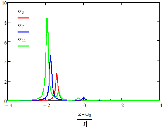
Absorption spectra for \(N=3,7,11\) for negative coupling.

The shift in the peak of the absorption relative to the monomer gives the coupling \(J\). Including long-range interactions has the effect of shifting the exciton band asymmetrically about \(\omega _ {0}\).

• \(\Omega _ {1} = \omega _ {0} + 2.4 J\) (\(m=1\), bottom of the band with \(J\) negative)
• \(\Omega _ {N} = \omega _ {0} - 1.8 J\) (Top of band)

Exchange Narrowing

If the chain is not homogeneous, i.e., all molecules do not have same site energy \(\varepsilon _ {0}\), then we can model this effect as Gaussian random disorder. The energy of a given site is

\[\varepsilon _ {n} = \varepsilon _ {0} + \delta \omega _ {n}\]

We add as an extra term to our earlier Hamiltonian, Equation \ref{14.30}, to account for this variation.

\[H _ {0} = H _ {s} + H _ {d i s} + V\]

\[H _ {d i s} = \sum _ {n} \delta \omega _ {n} | n \rangle \langle n |\]

The effect is to shift and mix the homogeneous exciton states. Absorption spectra for N = 3,7,11 for negative coupling

\[\delta \Omega _ {k} = \left\langle k \left| H _ {d i s} \right| k \right\rangle = \frac {2} {N + 1} \sum _ {n} \sin^{2} \left( \frac {\pi k n} {N + 1} \right) \delta \omega _ {n}\]

We find that these shifts are also Gaussian random variables, with a standard deviation of \(\Delta \sqrt {3 / 2 ( N + 1 )}\), where \(\Delta\) is the standard deviation for site energies. So, the delocalization of the eigenstate averages the disorder over \(N\) sites, which reduces the distribution of energies by a factor scaling as \(N\). The narrowing of the absorption lineshape with delocalization is called exchange narrowing. This depends on the distribution of site energies being relatively small: \(\Delta \ll 3 \pi | J | / N^{3 / 2}\).

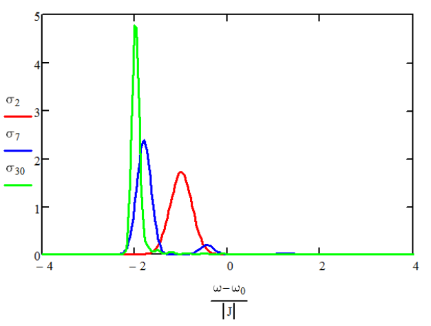
Absorption spectra for \(N =2,6,30\) normalized to the number of oscillators. \(3\Delta = J\) and \(J<0\).

Readings

1. Knoester, J., Optical Properties of Molecular Aggregates. In Proceedings of the International School of Physics "Enrico Fermi" Course CXLIX, Agranovich, M.; La Rocca, G. C., Eds. IOS Press: Amsterdam, 2002; pp 149-186.