13.2: Coupling to a Harmonic Bath

It is worth noting a similarity between the Hamiltonian for this displaced harmonic oscillator problem, and a general form for the interaction of an electronic “system” that is observed in an experiment with a harmonic oscillator “bath” whose degrees of freedom are invisible to the observable, but which influence the behavior of the system. This reasoning will in fact be developed more carefully later for the description of fluctuations. While the Hamiltonians we have written so far describe coupling to a single bath degree of freedom, the DHO model is readily generalized to many vibrations or a continuum of nuclear motions. Coupling to a continuum, or a harmonic bath, is the starting point for developing how an electronic system interacts with a continuum of intermolecular motions and phonons typical of condensed phase systems.

So, what happens if the electronic transition is coupled to many vibrational coordinates, each with its own displacement? The extension is straightforward if we still only consider two electronic states (\(e\) and \(g\)) to which we couple a set of independent modes, i.e., a bath of harmonic normal modes. Then we can write the Hamiltonian for \(N\) vibrations as a sum over all the independent harmonic modes

\[H _ {e} = \sum _ {\alpha = 1}^{N} H _ {e}^{( \alpha )} = \sum _ {\alpha = 1}^{N} \left( \frac {p _ {\alpha}^{2}} {2 m _ {\alpha}} + \frac {1} {2} m _ {\alpha} \omega _ {a}^{2} \left( q _ {\alpha} - d _ {\alpha} \right)^{2} \right) \label{12.49}\]

each with their distinct frequency and displacement. We can specify the state of the system in terms of product states in the electronic and nuclear occupation, i.e.,

\[\left.\begin{aligned} | G \rangle & = | g ; n _ {1} , n _ {2} , \ldots , n _ {N} \rangle \\ & = | g \rangle \prod _ {\alpha = 1}^{N} | n _ {\alpha} \rangle \end{aligned} \right. \label{12.50}\]

Additionally, we recognize that the time propagator on the electronic excited potential energy surface is

\[U _ {e} = \exp \left[ - \frac {i} {\hbar} H _ {e} t \right] = \prod _ {\alpha = 1}^{N} U _ {e}^{( \alpha )} \label{12.51}\]

where

\[U _ {e}^{( \alpha )} = \exp \left[ - \frac {i} {\hbar} H _ {e}^{( \alpha )} t \right] \label{12.52}\]

Defining \(D _ {\alpha} = d _ {\alpha}^{2} \left( m \omega _ {\alpha} / 2 \hbar \right)\)

\[\left.\begin{aligned} F^{( \alpha )} & = \left\langle \left[ U _ {g}^{( \alpha )} \right]^{\dagger} U _ {e}^{( \alpha )} \right\rangle \\ & = \exp \left[ D _ {\alpha} \left( e^{- i \omega _ {a} t} - 1 \right) \right] \end{aligned} \right. \label{12.53}\]

the dipole correlation function is then just a product of multiple dephasing functions that characterize the time-evolution of the different vibrations.

\[C _ {\mu \mu} (t) = \left| \mu _ {e g} \right|^{2} e^{- i \omega _ {e g} t} \cdot \prod _ {\alpha = 1}^{N} F^{( \alpha )} (t) \label{12.54}\]

or

\[C _ {\mu \mu} (t) = \left| \mu _ {e g} \right|^{2} e^{- i \omega _ {e g} t + g (t)} \label{12.55}\]

with

\[g (t) = \sum _ {\alpha} D _ {\alpha} \left( e^{- i \omega _ {a} t} - 1 \right) \label{12.56}\]

In the time domain this is a complex beating pattern, which in the frequency domain appears as a spectrum with several superimposed vibronic progressions that follow the rules developed above. Also, the reorganization energy now reflects to total excess nuclear potential energy required to make the electronic transition:

\[\lambda = \sum _ {\alpha} D _ {\alpha} \hbar \omega _ {\alpha} \label{12.57}\]

Taking this a step further, the generalization to a continuum of nuclear states emerges naturally. Given that we have a continuous frequency distribution of normal modes characterized by a density of states, \(W(\omega)\), and a continuously varying frequency-dependent coupling \(D ( \omega )\), we can change the sum in Equation \ref{12.56} to an integral over the density of states:

\[g (t) = \int d \omega \,W ( \omega ) D ( \omega ) \left( e^{- i \omega t} - 1 \right) \label{12.58}\]

Here the product \(W ( \omega )D ( \omega )\) is a coupling-weighted density of states, and is commonly referred to as a spectral density.

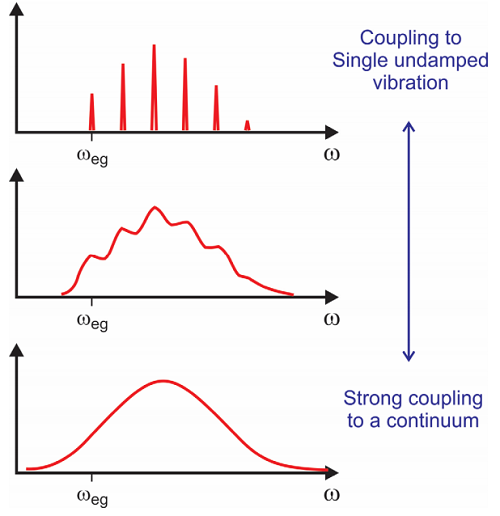
What this treatment does is provide a way of introducing a bath of states that the spectroscopically interrogated transition couples with. Coupling to a bath or continuum provides a way of introducing relaxation effects or damping of the electronic coherence in the absorption spectrum. You can see that if \(g(t)\) is associated with a constant \(\Gamma\), we obtain a Lorentzian lineshape with width \(\Gamma\). This emerges under certain circumstances, for instance if the distribution of states and coupling is large and constant, and if the integral in Equation \ref{12.58} is over a distribution of low frequencies, such that \(e^{- i \omega t} \approx 1 - i \omega t\). More generally the lineshape function is complex, and the real part describes damping and the imaginary part modulates the primary frequency and leads to fine structure. We will discuss these circumstances in more detail later.

An Ensemble at Finite Temperature

As described above, the single mode DHO model above is for a pure state, but the approach can be readily extended to describe a canonical ensemble. In this case, the correlation function is averaged over a thermal distribution of initial states. If we take the initial state of the system to be in the electronic ground state and its vibrational levels (\(n_g\)) to be occupied as a Boltzmann distribution, which is characteristic of ambient temperature samples, then the dipole correlation function can be written as a thermally averaged dephasing function:

\[C _ {\mu \mu} (t) = \left| \mu _ {e g} \right|^{2} e^{- i \omega _ {g} t} F (t) \label{12.59}\]

\[F (t) = \sum _ {n _ {g}} p \left( n _ {g} \right) \left\langle n _ {g} \left| U _ {g}^{\dagger} U _ {e} \right| n _ {g} \right\rangle \label{12.60}\]

\[p \left( n _ {g} \right) = \frac {e^{- \beta \ln a _ {b}}} {Z} \label{12.61}\]

Evaluating these expressions using the strategies developed above leads to

\[C _ {\mu \mu} (t) = \left| \mu _ {e g} \right|^{2} e^{- i \omega _ {e g} t} \exp \left[ D \left[ ( \overline {n} + 1 ) \left( e^{- i \omega _ {0} t} - 1 \right) + \overline {n} \left( e^{+ i \omega _ {0} t} - 1 \right) \right] \right\rceil \label{12.62}\]

\(\overline {n}\) is the thermally averaged occupation number of the harmonic vibrational mode.

\[\overline {n} = \left( e^{\beta \hbar \omega _ {0}} - 1 \right)^{- 1} \label{12.63}\]

Note that in the low temperature limit, \(\overline {n} \rightarrow 0\), and Equation \ref{12.62} equals our original result Equation \ref{12.32}. The dephasing function has two terms underlined in Equation \ref{12.62}, of which the first describes those electronic absorption events in which the vibrational quantum number increases or is unchanged (\(n_e≥n_g\)), whereas the second are for those processes where the vibrational quantum number decreases or is unchanged (\(n_e≤n_g\)). The latter are only allowed at elevated temperature where thermally excited states are populated and are known as “hot bands”.

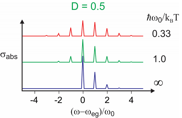
Now, let’s calculate the lineshape. If we separate the dephasing function into a product of two exponential terms and expand each of these exponentials, we can Fourier transform to give

\[\sigma _ {a b s} ( \omega ) = \left| \mu _ {e g} \right|^{2} e^{- D ( 2 \overline {n} + 1 )} \sum _ {j = 0}^{\infty} \sum _ {k = 0}^{\infty} \left( \frac {D^{j + k}} {j ! k !} \right) ( \overline {n} + 1 )^{j} \overline {n}^{k} \delta \left( \omega - \omega _ {e g} - ( j - k ) \omega _ {0} \right) \label{12.64}\]

Here the summation over \(j\) describes \(n_e≥n_g\) transitions, whereas the summation over \(k\) describes \(n_e≤n_g\). For any one transition frequency, (\(\omega \mathrm {eg}^{+} n \omega 0\)), the net absorption is a sum over all possible combination of transitions at the energy splitting with \(n=(j-k)\). Again, if we set \(\overline {n} \rightarrow 0\), we obtain our original result Equation 13.1.47. The contributions where \(k<j\) leads to the hot bands.

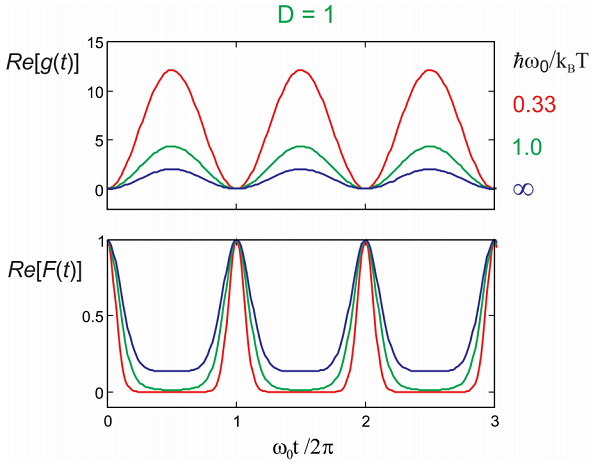
Examples of temperature dependence to lineshape and dephasing functions for \(D = 1\). The real part changes in amplitude, growing with temperature, whereas the imaginary part is unchanged.

We can extend this description to describe coupling to a many independent nuclear modes or coupling to a continuum. We write the state of the system in terms of the electronic state and the nuclear quantum numbers, i.e., \(| E \rangle = | e ; n _ {1} , n _ {2} , n _ {3} \dots \rangle\) and from that:

\[F (t) = \exp \left[ \sum _ {j} D _ {j} \left[ \left( \overline {n} _ {j} + 1 \right) \left( e^{- i \omega _ {j} t} - 1 \right) + \overline {n} _ {j} \left( e^{i \omega _ {j} t} - 1 \right) \right] \right] \label{12.65}\]

or changing to an integral over a continuous frequency distribution of normal modes characterized by a density of states, \(W(\omega)\)

\[F (t) = \exp \left[ \int d \omega \, W ( \omega ) D ( \omega ) \left[ ( \overline {n} ( \omega ) + 1 ) \left( e^{- i \omega t} - 1 \right) + \overline {n} ( \omega ) \left( e^{i \omega t} - 1 \right) \right] \right] \label{12.66}\]

\(D ( \omega )\) is the frequency dependent coupling. Let’s look at the envelope of the nuclear structure on the transition by doing a short-time expansion on the complex exponential as in Equation 13.1.49

\[F (t) = \exp \left[ \int d \omega \,D ( \omega ) W ( \omega ) \left( - i \omega t - ( 2 \overline {n} + 1 ) \frac {\omega^{2} t^{2}} {2} \right) \right] \label{12.67}\]

The lineshape is calculated from

\[\sigma _ {a b s} ( \omega ) = \int _ {- \infty}^{+ \infty} d t \,e^{i \left( \omega - \omega _ {e g} \right) t} \exp [ - i \langle \omega \rangle t ] \exp \left[ - \frac {1} {2} \left\langle \omega^{2} \right\rangle t^{2} \right] \label{12.68}\]

where we have defined the mean vibrational excitation on absorption

\[\begin{align} \langle \omega \rangle & = \int d \omega \, W ( \omega ) D ( \omega ) \omega \\[4pt] & = \lambda / \hbar \label{12.69} \end{align}\]

and

\[\left\langle \omega^{2} \right\rangle = \int d \omega\, W ( \omega ) D ( \omega ) \omega^{2} ( 2 \overline {n} ( \omega ) + 1 ) \label{12.70}\]

\(\left\langle \omega^{2} \right\rangle\) reflects the thermally averaged distribution of accessible vibrational states. Completing the square of Equation \ref{12.68} gives

\[\sigma _ {a b s} ( \omega ) = \left| \mu _ {e g} \right|^{2} \sqrt {\frac {2 \pi} {\left\langle \omega^{2} \right\rangle}} \exp \left[ \frac {- \left( \omega - \omega _ {e g} - \langle \omega \rangle \right)^{2}} {2 \left\langle \omega^{2} \right\rangle} \right] \label{12.71}\]

The lineshape is Gaussian, with a transition maximum at the electronic resonance plus reorganization energy. Although the frequency shift \(\langle \omega \rangle\) is not temperature dependent, the width of the Gaussian is temperature-dependent as a result of the thermal occupation factor in Equation \ref{12.70}.