
6.1: Born–Oppenheimer Approximation
- Page ID
- 107244

\( \newcommand{\vecs}[1]{\overset { \scriptstyle \rightharpoonup} {\mathbf{#1}} } \)
\( \newcommand{\vecd}[1]{\overset{-\!-\!\rightharpoonup}{\vphantom{a}\smash {#1}}} \)
\( \newcommand{\id}{\mathrm{id}}\) \( \newcommand{\Span}{\mathrm{span}}\)
( \newcommand{\kernel}{\mathrm{null}\,}\) \( \newcommand{\range}{\mathrm{range}\,}\)
\( \newcommand{\RealPart}{\mathrm{Re}}\) \( \newcommand{\ImaginaryPart}{\mathrm{Im}}\)
\( \newcommand{\Argument}{\mathrm{Arg}}\) \( \newcommand{\norm}[1]{\| #1 \|}\)
\( \newcommand{\inner}[2]{\langle #1, #2 \rangle}\)
\( \newcommand{\Span}{\mathrm{span}}\)
\( \newcommand{\id}{\mathrm{id}}\)
\( \newcommand{\Span}{\mathrm{span}}\)
\( \newcommand{\kernel}{\mathrm{null}\,}\)
\( \newcommand{\range}{\mathrm{range}\,}\)
\( \newcommand{\RealPart}{\mathrm{Re}}\)
\( \newcommand{\ImaginaryPart}{\mathrm{Im}}\)
\( \newcommand{\Argument}{\mathrm{Arg}}\)
\( \newcommand{\norm}[1]{\| #1 \|}\)
\( \newcommand{\inner}[2]{\langle #1, #2 \rangle}\)
\( \newcommand{\Span}{\mathrm{span}}\) \( \newcommand{\AA}{\unicode[.8,0]{x212B}}\)
\( \newcommand{\vectorA}[1]{\vec{#1}} % arrow\)
\( \newcommand{\vectorAt}[1]{\vec{\text{#1}}} % arrow\)
\( \newcommand{\vectorB}[1]{\overset { \scriptstyle \rightharpoonup} {\mathbf{#1}} } \)
\( \newcommand{\vectorC}[1]{\textbf{#1}} \)
\( \newcommand{\vectorD}[1]{\overrightarrow{#1}} \)
\( \newcommand{\vectorDt}[1]{\overrightarrow{\text{#1}}} \)
\( \newcommand{\vectE}[1]{\overset{-\!-\!\rightharpoonup}{\vphantom{a}\smash{\mathbf {#1}}}} \)
\( \newcommand{\vecs}[1]{\overset { \scriptstyle \rightharpoonup} {\mathbf{#1}} } \)
\( \newcommand{\vecd}[1]{\overset{-\!-\!\rightharpoonup}{\vphantom{a}\smash {#1}}} \)
\(\newcommand{\avec}{\mathbf a}\) \(\newcommand{\bvec}{\mathbf b}\) \(\newcommand{\cvec}{\mathbf c}\) \(\newcommand{\dvec}{\mathbf d}\) \(\newcommand{\dtil}{\widetilde{\mathbf d}}\) \(\newcommand{\evec}{\mathbf e}\) \(\newcommand{\fvec}{\mathbf f}\) \(\newcommand{\nvec}{\mathbf n}\) \(\newcommand{\pvec}{\mathbf p}\) \(\newcommand{\qvec}{\mathbf q}\) \(\newcommand{\svec}{\mathbf s}\) \(\newcommand{\tvec}{\mathbf t}\) \(\newcommand{\uvec}{\mathbf u}\) \(\newcommand{\vvec}{\mathbf v}\) \(\newcommand{\wvec}{\mathbf w}\) \(\newcommand{\xvec}{\mathbf x}\) \(\newcommand{\yvec}{\mathbf y}\) \(\newcommand{\zvec}{\mathbf z}\) \(\newcommand{\rvec}{\mathbf r}\) \(\newcommand{\mvec}{\mathbf m}\) \(\newcommand{\zerovec}{\mathbf 0}\) \(\newcommand{\onevec}{\mathbf 1}\) \(\newcommand{\real}{\mathbb R}\) \(\newcommand{\twovec}[2]{\left[\begin{array}{r}#1 \\ #2 \end{array}\right]}\) \(\newcommand{\ctwovec}[2]{\left[\begin{array}{c}#1 \\ #2 \end{array}\right]}\) \(\newcommand{\threevec}[3]{\left[\begin{array}{r}#1 \\ #2 \\ #3 \end{array}\right]}\) \(\newcommand{\cthreevec}[3]{\left[\begin{array}{c}#1 \\ #2 \\ #3 \end{array}\right]}\) \(\newcommand{\fourvec}[4]{\left[\begin{array}{r}#1 \\ #2 \\ #3 \\ #4 \end{array}\right]}\) \(\newcommand{\cfourvec}[4]{\left[\begin{array}{c}#1 \\ #2 \\ #3 \\ #4 \end{array}\right]}\) \(\newcommand{\fivevec}[5]{\left[\begin{array}{r}#1 \\ #2 \\ #3 \\ #4 \\ #5 \\ \end{array}\right]}\) \(\newcommand{\cfivevec}[5]{\left[\begin{array}{c}#1 \\ #2 \\ #3 \\ #4 \\ #5 \\ \end{array}\right]}\) \(\newcommand{\mattwo}[4]{\left[\begin{array}{rr}#1 \amp #2 \\ #3 \amp #4 \\ \end{array}\right]}\) \(\newcommand{\laspan}[1]{\text{Span}\{#1\}}\) \(\newcommand{\bcal}{\cal B}\) \(\newcommand{\ccal}{\cal C}\) \(\newcommand{\scal}{\cal S}\) \(\newcommand{\wcal}{\cal W}\) \(\newcommand{\ecal}{\cal E}\) \(\newcommand{\coords}[2]{\left\{#1\right\}_{#2}}\) \(\newcommand{\gray}[1]{\color{gray}{#1}}\) \(\newcommand{\lgray}[1]{\color{lightgray}{#1}}\) \(\newcommand{\rank}{\operatorname{rank}}\) \(\newcommand{\row}{\text{Row}}\) \(\newcommand{\col}{\text{Col}}\) \(\renewcommand{\row}{\text{Row}}\) \(\newcommand{\nul}{\text{Nul}}\) \(\newcommand{\var}{\text{Var}}\) \(\newcommand{\corr}{\text{corr}}\) \(\newcommand{\len}[1]{\left|#1\right|}\) \(\newcommand{\bbar}{\overline{\bvec}}\) \(\newcommand{\bhat}{\widehat{\bvec}}\) \(\newcommand{\bperp}{\bvec^\perp}\) \(\newcommand{\xhat}{\widehat{\xvec}}\) \(\newcommand{\vhat}{\widehat{\vvec}}\) \(\newcommand{\uhat}{\widehat{\uvec}}\) \(\newcommand{\what}{\widehat{\wvec}}\) \(\newcommand{\Sighat}{\widehat{\Sigma}}\) \(\newcommand{\lt}{<}\) \(\newcommand{\gt}{>}\) \(\newcommand{\amp}{&}\) \(\definecolor{fillinmathshade}{gray}{0.9}\)As a starting point, it is helpful to review the Born–Oppenheimer Approximation (BOA). For a molecular system, the Hamiltonian can be written in terms of the kinetic energy of the nuclei (\(N\)) and electrons (\(e\)) and the potential energy for the Coulomb interactions of these particles.
\[\begin{align} \hat {H} = \hat {T} _ {e} + \hat {T} _ {N} + \hat {V} _ {e e} + \hat {V} _ {N N} + \hat {V} _ {e N} \\[4pt] = - \sum _ {i = 1}^{n} \frac {\hbar^{2}} {2 m _ {e}} \nabla _ {i}^{2} - \sum _ {J = 1}^{N} \frac {\hbar^{2}} {2 M _ {J}} \nabla _ {J}^{2} \\[4pt] = - \sum _ {i = 1}^{n} \frac {\hbar^{2}} {2 m _ {e}} \nabla _ {i}^{2} - \sum _ {J = 1}^{N} \frac {\hbar^{2}} {2 M _ {J}} \nabla _ {J}^{2} \label{5.1} \end{align}\]
Here and in the following, we will use lowercase variables to refer to electrons and uppercase to nuclei. The variables \(n\), \(i\), \(\mathbf {r}\), \(\nabla _ {r}^{2}\), and \(m_e\) refer to the number, index, position, Laplacian, and mass of electrons, respectively, and \(N\), \(J\), \(\mathbf {R}\), and \(M\) refer to the nuclei. \(e\) is the electron charge, and \(Z\) is the atomic number of the nucleus. Note, this Hamiltonian does not include relativistic effects such as spin-orbit coupling.
The time-independent Schrödinger equation is
\[\hat {H} ( \hat {\mathbf {r}} , \hat {\mathbf {R}} ) \Psi ( \hat {\mathbf {r}} , \hat {\mathbf {R}} ) = E \Psi ( \hat {\mathbf {r}} , \hat {\mathbf {R}} ) \label{5.2}\]
\(\Psi ( \hat {\mathbf {r}} , \hat {\mathbf {R}} )\) is the total vibronic wavefunction, where “vibronic” refers to the combined electronic and nuclear eigenstates. Exact solutions using the molecular Hamiltonian are intractable for most problems of interest, so we turn to simplifying approximations. The BO approximation is motivated by noting that the nuclei are far more massive than an electron (\(m_e \ll M_I\)). With this criterion, and when the distances separating particles is not unusually small, the kinetic energy of the nuclei is small relative to the other terms in the Hamiltonian. Physically, this means that the electrons move and adapt rapidly—adiabatically—in response to shifting nuclear positions. This offers an avenue to solving for \(\Psi\) by fixing the position of the nuclei, solving for the electronic wavefunctions \(\psi_i\), and then iterating for varying \(\boldsymbol {R}\) to obtain effective electronic potentials on which the nuclei move.
Since it is fixed for the electronic calculation, we proceed by treating \(\mathbf {R}\) as a parameter rather than an operator, set \(\hat{T}_N\) to 0, and solve the electronic TISE:
\[\hat {H} _ {e l} ( \hat {\mathbf {r}} , \mathbf {R} ) \psi _ {i} ( \hat {\mathbf {r}} , \mathbf {R} ) = U _ {i} ( \mathbf {R} ) \psi _ {i} ( \hat {\mathbf {r}} , \mathbf {R} ) \label{5.3}\]
\(U_i\) are the electronic energy eigenvalues for the fixed nuclei, and the electronic Hamiltonian in the BO approximation is
\[\hat {H} _ {e l} = \hat {T} _ {e} + \hat {V} _ {e e} + \hat {V} _ {e N} \label{5.4}\]
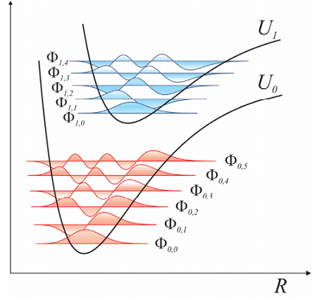
In Equation \ref{5.3}, \(\psi_i\) is the electronic wavefunction for fixed \(\mathbf {R}\), with \(i = 0\) referring to the electronic ground state. Repeating this calculation for varying \(\mathbf {R}\), we obtain \(U_i(R)\), an effective or mean-field potential for the electronic states on which the nuclei can move. These effective potentials are known as Born–Oppenheimer or adiabatic potential energy surfaces (PES).
For the nuclear degrees of freedom, we can define a Hamiltonian for the ith electronic PES: ,
\[\hat {H} _ {N u c , i} = \hat {T} _ {N} + U _ {i} ( \hat {R} ) \label{5.5}\]
which satisfies a TISE for the nuclear wave functions \(\Phi(R)\) :
\[\hat {H} _ {N u c , i} \Phi _ {i J} ( R ) = E _ {i J} \Phi _ {i J} ( R ) \label{5.6}\]
Here \(J\) refers to the Jth eigenstate for nuclei evolving on the i th PES. Equation \ref{5.5} is referred to as the BO Hamiltonian.
The BOA effectively separates the nuclear and electronic contributions to the wavefunction, allowing us to express the total wavefunction as a product of these contributions
\[\Psi ( \mathbf {r} , \mathbf {R} ) = \Phi ( \mathbf {R} ) \psi ( \mathbf {r} , \mathbf {R} )\] and the eigenvalues as sums over the electronic and nuclear contribution:
\(E = E _ {N} + E _ {e}.\) BOA does not treat the nuclei classically. However, it is the basis for semiclassical dynamics methods in which the nuclei evolve classically on a potential energy surface, and interact with quantum electronic states. If we treat the nuclear dynamics classically, then the electronic Hamiltonian can be thought of as depending on \(\mathbf {R}\) or on time as related by velocity or momenta. If the nuclei move infinitely slowly, the electrons will adiabatically follow the nuclei and systems prepared in an electronic eigenstate will remain in that eigenstate for all times.