15.6: Chemical Potential, Fugacity, and Equilibrium
- Page ID
- 151758
\( \newcommand{\vecs}[1]{\overset { \scriptstyle \rightharpoonup} {\mathbf{#1}} } \)
\( \newcommand{\vecd}[1]{\overset{-\!-\!\rightharpoonup}{\vphantom{a}\smash {#1}}} \)
\( \newcommand{\id}{\mathrm{id}}\) \( \newcommand{\Span}{\mathrm{span}}\)
( \newcommand{\kernel}{\mathrm{null}\,}\) \( \newcommand{\range}{\mathrm{range}\,}\)
\( \newcommand{\RealPart}{\mathrm{Re}}\) \( \newcommand{\ImaginaryPart}{\mathrm{Im}}\)
\( \newcommand{\Argument}{\mathrm{Arg}}\) \( \newcommand{\norm}[1]{\| #1 \|}\)
\( \newcommand{\inner}[2]{\langle #1, #2 \rangle}\)
\( \newcommand{\Span}{\mathrm{span}}\)
\( \newcommand{\id}{\mathrm{id}}\)
\( \newcommand{\Span}{\mathrm{span}}\)
\( \newcommand{\kernel}{\mathrm{null}\,}\)
\( \newcommand{\range}{\mathrm{range}\,}\)
\( \newcommand{\RealPart}{\mathrm{Re}}\)
\( \newcommand{\ImaginaryPart}{\mathrm{Im}}\)
\( \newcommand{\Argument}{\mathrm{Arg}}\)
\( \newcommand{\norm}[1]{\| #1 \|}\)
\( \newcommand{\inner}[2]{\langle #1, #2 \rangle}\)
\( \newcommand{\Span}{\mathrm{span}}\) \( \newcommand{\AA}{\unicode[.8,0]{x212B}}\)
\( \newcommand{\vectorA}[1]{\vec{#1}} % arrow\)
\( \newcommand{\vectorAt}[1]{\vec{\text{#1}}} % arrow\)
\( \newcommand{\vectorB}[1]{\overset { \scriptstyle \rightharpoonup} {\mathbf{#1}} } \)
\( \newcommand{\vectorC}[1]{\textbf{#1}} \)
\( \newcommand{\vectorD}[1]{\overrightarrow{#1}} \)
\( \newcommand{\vectorDt}[1]{\overrightarrow{\text{#1}}} \)
\( \newcommand{\vectE}[1]{\overset{-\!-\!\rightharpoonup}{\vphantom{a}\smash{\mathbf {#1}}}} \)
\( \newcommand{\vecs}[1]{\overset { \scriptstyle \rightharpoonup} {\mathbf{#1}} } \)
\( \newcommand{\vecd}[1]{\overset{-\!-\!\rightharpoonup}{\vphantom{a}\smash {#1}}} \)
\(\newcommand{\avec}{\mathbf a}\) \(\newcommand{\bvec}{\mathbf b}\) \(\newcommand{\cvec}{\mathbf c}\) \(\newcommand{\dvec}{\mathbf d}\) \(\newcommand{\dtil}{\widetilde{\mathbf d}}\) \(\newcommand{\evec}{\mathbf e}\) \(\newcommand{\fvec}{\mathbf f}\) \(\newcommand{\nvec}{\mathbf n}\) \(\newcommand{\pvec}{\mathbf p}\) \(\newcommand{\qvec}{\mathbf q}\) \(\newcommand{\svec}{\mathbf s}\) \(\newcommand{\tvec}{\mathbf t}\) \(\newcommand{\uvec}{\mathbf u}\) \(\newcommand{\vvec}{\mathbf v}\) \(\newcommand{\wvec}{\mathbf w}\) \(\newcommand{\xvec}{\mathbf x}\) \(\newcommand{\yvec}{\mathbf y}\) \(\newcommand{\zvec}{\mathbf z}\) \(\newcommand{\rvec}{\mathbf r}\) \(\newcommand{\mvec}{\mathbf m}\) \(\newcommand{\zerovec}{\mathbf 0}\) \(\newcommand{\onevec}{\mathbf 1}\) \(\newcommand{\real}{\mathbb R}\) \(\newcommand{\twovec}[2]{\left[\begin{array}{r}#1 \\ #2 \end{array}\right]}\) \(\newcommand{\ctwovec}[2]{\left[\begin{array}{c}#1 \\ #2 \end{array}\right]}\) \(\newcommand{\threevec}[3]{\left[\begin{array}{r}#1 \\ #2 \\ #3 \end{array}\right]}\) \(\newcommand{\cthreevec}[3]{\left[\begin{array}{c}#1 \\ #2 \\ #3 \end{array}\right]}\) \(\newcommand{\fourvec}[4]{\left[\begin{array}{r}#1 \\ #2 \\ #3 \\ #4 \end{array}\right]}\) \(\newcommand{\cfourvec}[4]{\left[\begin{array}{c}#1 \\ #2 \\ #3 \\ #4 \end{array}\right]}\) \(\newcommand{\fivevec}[5]{\left[\begin{array}{r}#1 \\ #2 \\ #3 \\ #4 \\ #5 \\ \end{array}\right]}\) \(\newcommand{\cfivevec}[5]{\left[\begin{array}{c}#1 \\ #2 \\ #3 \\ #4 \\ #5 \\ \end{array}\right]}\) \(\newcommand{\mattwo}[4]{\left[\begin{array}{rr}#1 \amp #2 \\ #3 \amp #4 \\ \end{array}\right]}\) \(\newcommand{\laspan}[1]{\text{Span}\{#1\}}\) \(\newcommand{\bcal}{\cal B}\) \(\newcommand{\ccal}{\cal C}\) \(\newcommand{\scal}{\cal S}\) \(\newcommand{\wcal}{\cal W}\) \(\newcommand{\ecal}{\cal E}\) \(\newcommand{\coords}[2]{\left\{#1\right\}_{#2}}\) \(\newcommand{\gray}[1]{\color{gray}{#1}}\) \(\newcommand{\lgray}[1]{\color{lightgray}{#1}}\) \(\newcommand{\rank}{\operatorname{rank}}\) \(\newcommand{\row}{\text{Row}}\) \(\newcommand{\col}{\text{Col}}\) \(\renewcommand{\row}{\text{Row}}\) \(\newcommand{\nul}{\text{Nul}}\) \(\newcommand{\var}{\text{Var}}\) \(\newcommand{\corr}{\text{corr}}\) \(\newcommand{\len}[1]{\left|#1\right|}\) \(\newcommand{\bbar}{\overline{\bvec}}\) \(\newcommand{\bhat}{\widehat{\bvec}}\) \(\newcommand{\bperp}{\bvec^\perp}\) \(\newcommand{\xhat}{\widehat{\xvec}}\) \(\newcommand{\vhat}{\widehat{\vvec}}\) \(\newcommand{\uhat}{\widehat{\uvec}}\) \(\newcommand{\what}{\widehat{\wvec}}\) \(\newcommand{\Sighat}{\widehat{\Sigma}}\) \(\newcommand{\lt}{<}\) \(\newcommand{\gt}{>}\) \(\newcommand{\amp}{&}\) \(\definecolor{fillinmathshade}{gray}{0.9}\)In Chapter 13, we develop the relationship between the standard Gibbs free energy change for a reaction and the equilibrium constant for that reaction, under the assumption that all of the substances involved in the reaction behave ideally. In the gas phase, they behave as ideal gases; when dissolved in a solution, their concentrations are proportional to their mole fractions in a gas phase at equilibrium with the solution.
We can now repeat this development using the fugacities instead of the pressures of the reacting species. Let the reaction be
\[aA+bB\to cC+dD. \nonumber \]
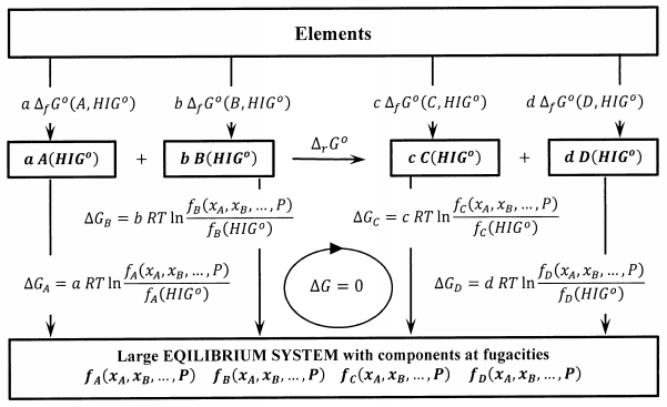
We introduce the reactions that create the reactants and the products in their hypothetical ideal-gas standard states from their elements in their standard states. The Gibbs free energy change for creating the reactants in their hypothetical ideal-gas standard states from the elements in their standard states is
\[a{\Delta }_fG^o\left(A,{HIG}^o\right)+b{\Delta }_fG^o\left(B,{HIG}^o\right) \nonumber \]
The Gibbs free energy change for creating the products in their standard states, from the same set of elements, is
\[c{\Delta }_fG^o\left(C,{HIG}^o\right)+d{\Delta }_fG^o\left(D,{HIG}^o\right) \nonumber \]
Next, we introduce a set of processes, each of which adds a further quantity of a reactant or product to a very large system at equilibrium. That is, we transfer an additional \(a\) moles of pure \(A\) from its hypothetical ideal-gas standard state into a very large system in which its fugacity is \(f_A\left(P,T,x_A,x_B,\dots .\right)\). The Gibbs free energy change for this process is
\[a\ RT{ \ln \left[\frac{f_A\left(P,T,x_A,x_B,\dots .\right)}{f_A\left({HIG}^o\right)}\right]\ } \nonumber \]
Corresponding processes add \(b\) moles of pure \(B\) at fugacity \(f_B\left(P,T,x_A,x_B,\dots .\right)\), etc. These processes are diagrammed in Figure 2. Since the fugacity of a substance in any state is a rigorous measure of the difference between its chemical potential in that state and its chemical potential in its hypothetical ideal-gas standard state, these Gibbs free energy changes are exact. Since the very large system is at equilibrium, there is no Gibbs free energy change when a moles of \(A\) and \(b\) moles of \(B\) react according to \(aA+bB\to cC+dD\).

Let us compute the Gibbs free energy change in a clockwise direction around the reversible cycle in Figure 2. The elements in their standard states are converted first to isolated products, then to components of the large equilibrium system, then to separated reactants, and finally back to the elements in their standard states. We have
\[0=c\ {\Delta }_fG^o\left(C,{HIG}^o\right)+d\ {\Delta }_fG^o\left(D,{HIG}^o\right)-a\ {\Delta }_fG^o\left(A,{HIG}^o\right)-b\ {\Delta }_fG^o\left(B,{HIG}^o\right)+c\ RT{ \ln \left[\frac{f_C\left(P,T,x_A,x_B,\dots .\right)}{f_C\left({HIG}^o\right)}\right]\ }+d\ RT{ \ln \left[\frac{f_D\left(P,T,x_A,x_B,\dots .\right)}{f_D\left({HIG}^o\right)}\right]\ }-a\ RT{ \ln \left[\frac{f_A\left(P,T,x_A,x_B,\dots .\right)}{f_A\left({HIG}^o\right)}\right]\ }-b\ RT{ \ln \left[\frac{f_B\left(P,T,x_A,x_B,\dots .\right)}{f_B\left({HIG}^o\right)}\right]\ } \nonumber \]
To express the fugacity ratios more compactly, we let
\[f_A=\frac{f_A\left(P,T,x_A,x_B,\dots .\right)}{f_A\left({HIG}^o\right)} \nonumber \]
etc. Letting
\[{\Delta }_rG^o=c\ {\Delta }_fG^o\left(C,{HIG}^o\right)+d\ {\Delta }_fG^o\left(D,{HIG}^o\right)-a\ {\Delta }_fG^o\left(A,{HIG}^o\right)-b\ {\Delta }_fG^o\left(B,{HIG}^o\right) \nonumber \]
the Gibbs free energy around this reversible cycle simplifies to \[{\Delta }_rG^o=-RT{ \ln \frac{f^c_Cf^d_D}{f^a_Af^b_B}\ } \nonumber \]
We can express the criterion for equilibrium as
\[K_f=\frac{f^c_Cf^d_D}{f^a_Af^b_B} \nonumber \]
where
\[K_f=\mathrm{exp}\left(\frac{-{\Delta }_rG^o}{RT}\right) \nonumber \]
We introduce the subscript, “\(f\)”, to indicate that the equilibrium constant, \(K_f\), is a function of the fugacities of the reacting substances. These relationships parallel those that we found for equilibrium among ideal gases, with real-gas fugacities replacing ideal-gas pressures.
As we did when we considered ideal-gas equilibria, let us suppose that the very large equilibrium system contains a liquid phase in which the reactants and products are soluble. The reaction can also occur in this liquid phase, and this liquid-phase reaction must be at equilibrium. Since the system is at equilibrium, each chemical species must have the same chemical potential in the solution as it does in the gas phase. Hence, the fugacities and the fugacity-based equilibrium constant are the same in both phases.
At this point, we have obtained—in principle—a complete solution to the problem of predicting the equilibrium position for any reaction. If we can find the Gibbs free energy of formation of each substance in its hypothetical ideal-gas standard state, and we can find its fugacity as a function of the composition and pressure of the system in which the reaction occurs, we can find the equilibrium constant and the equilibrium composition of the system.
In practice, a great many substances are non-volatile. The Gibbs free energy of formation of their hypothetical ideal-gas standard states and their fugacities cannot be measured. For such substances, we have recourse to other standard states and use activities to express the equilibrium constant.


