10.8: Using the Pair (V, P) or the Pair (T, S) as Independent Variables
- Page ID
- 152338
\( \newcommand{\vecs}[1]{\overset { \scriptstyle \rightharpoonup} {\mathbf{#1}} } \)
\( \newcommand{\vecd}[1]{\overset{-\!-\!\rightharpoonup}{\vphantom{a}\smash {#1}}} \)
\( \newcommand{\id}{\mathrm{id}}\) \( \newcommand{\Span}{\mathrm{span}}\)
( \newcommand{\kernel}{\mathrm{null}\,}\) \( \newcommand{\range}{\mathrm{range}\,}\)
\( \newcommand{\RealPart}{\mathrm{Re}}\) \( \newcommand{\ImaginaryPart}{\mathrm{Im}}\)
\( \newcommand{\Argument}{\mathrm{Arg}}\) \( \newcommand{\norm}[1]{\| #1 \|}\)
\( \newcommand{\inner}[2]{\langle #1, #2 \rangle}\)
\( \newcommand{\Span}{\mathrm{span}}\)
\( \newcommand{\id}{\mathrm{id}}\)
\( \newcommand{\Span}{\mathrm{span}}\)
\( \newcommand{\kernel}{\mathrm{null}\,}\)
\( \newcommand{\range}{\mathrm{range}\,}\)
\( \newcommand{\RealPart}{\mathrm{Re}}\)
\( \newcommand{\ImaginaryPart}{\mathrm{Im}}\)
\( \newcommand{\Argument}{\mathrm{Arg}}\)
\( \newcommand{\norm}[1]{\| #1 \|}\)
\( \newcommand{\inner}[2]{\langle #1, #2 \rangle}\)
\( \newcommand{\Span}{\mathrm{span}}\) \( \newcommand{\AA}{\unicode[.8,0]{x212B}}\)
\( \newcommand{\vectorA}[1]{\vec{#1}} % arrow\)
\( \newcommand{\vectorAt}[1]{\vec{\text{#1}}} % arrow\)
\( \newcommand{\vectorB}[1]{\overset { \scriptstyle \rightharpoonup} {\mathbf{#1}} } \)
\( \newcommand{\vectorC}[1]{\textbf{#1}} \)
\( \newcommand{\vectorD}[1]{\overrightarrow{#1}} \)
\( \newcommand{\vectorDt}[1]{\overrightarrow{\text{#1}}} \)
\( \newcommand{\vectE}[1]{\overset{-\!-\!\rightharpoonup}{\vphantom{a}\smash{\mathbf {#1}}}} \)
\( \newcommand{\vecs}[1]{\overset { \scriptstyle \rightharpoonup} {\mathbf{#1}} } \)
\( \newcommand{\vecd}[1]{\overset{-\!-\!\rightharpoonup}{\vphantom{a}\smash {#1}}} \)
\(\newcommand{\avec}{\mathbf a}\) \(\newcommand{\bvec}{\mathbf b}\) \(\newcommand{\cvec}{\mathbf c}\) \(\newcommand{\dvec}{\mathbf d}\) \(\newcommand{\dtil}{\widetilde{\mathbf d}}\) \(\newcommand{\evec}{\mathbf e}\) \(\newcommand{\fvec}{\mathbf f}\) \(\newcommand{\nvec}{\mathbf n}\) \(\newcommand{\pvec}{\mathbf p}\) \(\newcommand{\qvec}{\mathbf q}\) \(\newcommand{\svec}{\mathbf s}\) \(\newcommand{\tvec}{\mathbf t}\) \(\newcommand{\uvec}{\mathbf u}\) \(\newcommand{\vvec}{\mathbf v}\) \(\newcommand{\wvec}{\mathbf w}\) \(\newcommand{\xvec}{\mathbf x}\) \(\newcommand{\yvec}{\mathbf y}\) \(\newcommand{\zvec}{\mathbf z}\) \(\newcommand{\rvec}{\mathbf r}\) \(\newcommand{\mvec}{\mathbf m}\) \(\newcommand{\zerovec}{\mathbf 0}\) \(\newcommand{\onevec}{\mathbf 1}\) \(\newcommand{\real}{\mathbb R}\) \(\newcommand{\twovec}[2]{\left[\begin{array}{r}#1 \\ #2 \end{array}\right]}\) \(\newcommand{\ctwovec}[2]{\left[\begin{array}{c}#1 \\ #2 \end{array}\right]}\) \(\newcommand{\threevec}[3]{\left[\begin{array}{r}#1 \\ #2 \\ #3 \end{array}\right]}\) \(\newcommand{\cthreevec}[3]{\left[\begin{array}{c}#1 \\ #2 \\ #3 \end{array}\right]}\) \(\newcommand{\fourvec}[4]{\left[\begin{array}{r}#1 \\ #2 \\ #3 \\ #4 \end{array}\right]}\) \(\newcommand{\cfourvec}[4]{\left[\begin{array}{c}#1 \\ #2 \\ #3 \\ #4 \end{array}\right]}\) \(\newcommand{\fivevec}[5]{\left[\begin{array}{r}#1 \\ #2 \\ #3 \\ #4 \\ #5 \\ \end{array}\right]}\) \(\newcommand{\cfivevec}[5]{\left[\begin{array}{c}#1 \\ #2 \\ #3 \\ #4 \\ #5 \\ \end{array}\right]}\) \(\newcommand{\mattwo}[4]{\left[\begin{array}{rr}#1 \amp #2 \\ #3 \amp #4 \\ \end{array}\right]}\) \(\newcommand{\laspan}[1]{\text{Span}\{#1\}}\) \(\newcommand{\bcal}{\cal B}\) \(\newcommand{\ccal}{\cal C}\) \(\newcommand{\scal}{\cal S}\) \(\newcommand{\wcal}{\cal W}\) \(\newcommand{\ecal}{\cal E}\) \(\newcommand{\coords}[2]{\left\{#1\right\}_{#2}}\) \(\newcommand{\gray}[1]{\color{gray}{#1}}\) \(\newcommand{\lgray}[1]{\color{lightgray}{#1}}\) \(\newcommand{\rank}{\operatorname{rank}}\) \(\newcommand{\row}{\text{Row}}\) \(\newcommand{\col}{\text{Col}}\) \(\renewcommand{\row}{\text{Row}}\) \(\newcommand{\nul}{\text{Nul}}\) \(\newcommand{\var}{\text{Var}}\) \(\newcommand{\corr}{\text{corr}}\) \(\newcommand{\len}[1]{\left|#1\right|}\) \(\newcommand{\bbar}{\overline{\bvec}}\) \(\newcommand{\bhat}{\widehat{\bvec}}\) \(\newcommand{\bperp}{\bvec^\perp}\) \(\newcommand{\xhat}{\widehat{\xvec}}\) \(\newcommand{\vhat}{\widehat{\vvec}}\) \(\newcommand{\uhat}{\widehat{\uvec}}\) \(\newcommand{\what}{\widehat{\wvec}}\) \(\newcommand{\Sighat}{\widehat{\Sigma}}\) \(\newcommand{\lt}{<}\) \(\newcommand{\gt}{>}\) \(\newcommand{\amp}{&}\) \(\definecolor{fillinmathshade}{gray}{0.9}\)When only pressure–volume work is possible, various pairs of state functions can specify the state of any closed equilibrium system. A given pair may be sufficient to specify the state on a given Gibbsian manifold but not to specify the state of the same system on a different Gibbsian manifold. (In Section 10.7, we see that the set \(\left\{T,P\right\}\) is sufficient to specify the state of a closed system containing only liquid water or only gaseous water. However, specifying T and P is not sufficient to establish the amount of water vapor in a closed system in which the liquid is vaporizing reversibly.)
It can also happen that a given pair of state functions specifies the state of a closed system over part but not all of a given Gibbsian manifold. Specifying the values of such a pair is not sufficient to describe the entire manifold. In particular, we can show that neither the set \(\left\{P,V\right\}\) nor the set \(\left\{T,S\right\}\) is always a sufficient pair in this sense.
When we say that specifying \(P\) and \(V\) is sufficient to specify the state of a system on a particular Gibbsian manifold, we mean that any state function, \(M\), must be uniquely specified when \(P\) and \(V\) are specified; a single-valued function, \(M\left(P,V\right)\), must exist. Conversely, if for any choice of \(M\) in any system, \(M\left(P,V\right)\) is not single-valued,\(\ P\) and \(V\) are not always a sufficient set. In §6, we see how to find the total differential, \[dM={\left(\frac{\partial M}{\partial P}\right)}_VdP+{\left(\frac{\partial M}{\partial V}\right)}_PdV \nonumber \]
It might seem that this is sufficient to ensure that specifying P and V always enables us to find \(M\left(P,V\right)\) relative to its value in an initial reference state \(M\left(P_1,V_1\right)\). To do so, we need only evaluate \(dM\) as a line integral along some reversible path that leads from \(\left(P_1,V_1\right)\) to \(\left(P_2,V_2\right)\). However, we can evaluate this line integral only if both of the partial derivatives can be integrated. If one of the partial derivatives is undefined along any path that connects \(\left(P_1,V_1\right)\) to \(\left(P_2,V_2\right)\), we cannot find \(M\left(P,V\right)\) by this method.

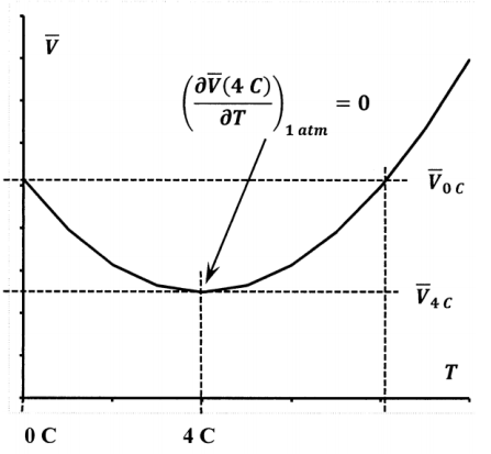
Let us consider a closed reversible system that consists of one mole of liquid water. At ordinary pressures, the density of liquid water is not a monotonic function of temperature. At one atmosphere, the density of liquid water reaches a maximum at 4 C. Therefore, at a pressure of one atmosphere, the molar volume of water is a minimum at 4 C, as indicated in Figure 2. This means that, at one atmosphere and a range of volumes, liquid water can be at either of two temperatures for specified values of \(P\) and \(\overline{V}\). Therefore, specifying \(P\) and \(\overline{V}\) does not specify \(T\); temperature is not a single-valued function of pressure and volume; we cannot uniquely express the temperature as the required function \(T=T\left(P,\overline{V}\right)\). Moreover, because the density has a maximum, we have
\[{\left(\frac{\partial \overline{V}}{\partial T}\right)}_P=0 \nonumber \]
at this maximum, and it follows that
\[{\left(\frac{\partial T}{\partial \overline{V}}\right)}_P \nonumber \]
is not defined at this temperature and pressure. In Section 10.6, we find
\[{\left(\frac{\partial \overline{S}}{\partial \overline{V}}\right)}_P={\frac{C_P}{T}\left(\frac{\partial T}{\partial \overline{V}}\right)}_P \nonumber \] so that \({\left({\partial \overline{S}}/{\partial \overline{V}}\right)}_P\) is also undefined. Hence, we cannot evaluate \(\Delta \overline{S}\) by evaluating the line integral of \(d\overline{S}\left(P,\overline{V}\right)\) along any path that includes a point of maximum density. These examples show that pressure and volume are not sufficient to describe the entire Gibbsian manifold for liquid water.
Temperature and entropy are likewise not sufficient. Since we have
\[d\overline{S} = \frac{C_P}{T}dT + {\left(\frac{\partial \overline{V}}{\partial T}\right)}_PdP \nonumber \]
the total differential for pressure as a function of entropy and temperature is
\[dP = \left[\frac{C_P}{T}dT + d\overline{S}\right]{\left(\frac{\partial T}{\partial \overline{V}}\right)}_P \nonumber \]
so that \(dP\) is not defined at pressures and temperatures of maximum density. Consequently, we cannot express the pressure as \(P=P\left(\overline{S},T\right)\) over the entire liquid region.


