
9.4: The Entropy Change around Any Cycle for Any Reversible System
- Page ID
- 151714

\( \newcommand{\vecs}[1]{\overset { \scriptstyle \rightharpoonup} {\mathbf{#1}} } \)
\( \newcommand{\vecd}[1]{\overset{-\!-\!\rightharpoonup}{\vphantom{a}\smash {#1}}} \)
\( \newcommand{\id}{\mathrm{id}}\) \( \newcommand{\Span}{\mathrm{span}}\)
( \newcommand{\kernel}{\mathrm{null}\,}\) \( \newcommand{\range}{\mathrm{range}\,}\)
\( \newcommand{\RealPart}{\mathrm{Re}}\) \( \newcommand{\ImaginaryPart}{\mathrm{Im}}\)
\( \newcommand{\Argument}{\mathrm{Arg}}\) \( \newcommand{\norm}[1]{\| #1 \|}\)
\( \newcommand{\inner}[2]{\langle #1, #2 \rangle}\)
\( \newcommand{\Span}{\mathrm{span}}\)
\( \newcommand{\id}{\mathrm{id}}\)
\( \newcommand{\Span}{\mathrm{span}}\)
\( \newcommand{\kernel}{\mathrm{null}\,}\)
\( \newcommand{\range}{\mathrm{range}\,}\)
\( \newcommand{\RealPart}{\mathrm{Re}}\)
\( \newcommand{\ImaginaryPart}{\mathrm{Im}}\)
\( \newcommand{\Argument}{\mathrm{Arg}}\)
\( \newcommand{\norm}[1]{\| #1 \|}\)
\( \newcommand{\inner}[2]{\langle #1, #2 \rangle}\)
\( \newcommand{\Span}{\mathrm{span}}\) \( \newcommand{\AA}{\unicode[.8,0]{x212B}}\)
\( \newcommand{\vectorA}[1]{\vec{#1}} % arrow\)
\( \newcommand{\vectorAt}[1]{\vec{\text{#1}}} % arrow\)
\( \newcommand{\vectorB}[1]{\overset { \scriptstyle \rightharpoonup} {\mathbf{#1}} } \)
\( \newcommand{\vectorC}[1]{\textbf{#1}} \)
\( \newcommand{\vectorD}[1]{\overrightarrow{#1}} \)
\( \newcommand{\vectorDt}[1]{\overrightarrow{\text{#1}}} \)
\( \newcommand{\vectE}[1]{\overset{-\!-\!\rightharpoonup}{\vphantom{a}\smash{\mathbf {#1}}}} \)
\( \newcommand{\vecs}[1]{\overset { \scriptstyle \rightharpoonup} {\mathbf{#1}} } \)
\( \newcommand{\vecd}[1]{\overset{-\!-\!\rightharpoonup}{\vphantom{a}\smash {#1}}} \)
\(\newcommand{\avec}{\mathbf a}\) \(\newcommand{\bvec}{\mathbf b}\) \(\newcommand{\cvec}{\mathbf c}\) \(\newcommand{\dvec}{\mathbf d}\) \(\newcommand{\dtil}{\widetilde{\mathbf d}}\) \(\newcommand{\evec}{\mathbf e}\) \(\newcommand{\fvec}{\mathbf f}\) \(\newcommand{\nvec}{\mathbf n}\) \(\newcommand{\pvec}{\mathbf p}\) \(\newcommand{\qvec}{\mathbf q}\) \(\newcommand{\svec}{\mathbf s}\) \(\newcommand{\tvec}{\mathbf t}\) \(\newcommand{\uvec}{\mathbf u}\) \(\newcommand{\vvec}{\mathbf v}\) \(\newcommand{\wvec}{\mathbf w}\) \(\newcommand{\xvec}{\mathbf x}\) \(\newcommand{\yvec}{\mathbf y}\) \(\newcommand{\zvec}{\mathbf z}\) \(\newcommand{\rvec}{\mathbf r}\) \(\newcommand{\mvec}{\mathbf m}\) \(\newcommand{\zerovec}{\mathbf 0}\) \(\newcommand{\onevec}{\mathbf 1}\) \(\newcommand{\real}{\mathbb R}\) \(\newcommand{\twovec}[2]{\left[\begin{array}{r}#1 \\ #2 \end{array}\right]}\) \(\newcommand{\ctwovec}[2]{\left[\begin{array}{c}#1 \\ #2 \end{array}\right]}\) \(\newcommand{\threevec}[3]{\left[\begin{array}{r}#1 \\ #2 \\ #3 \end{array}\right]}\) \(\newcommand{\cthreevec}[3]{\left[\begin{array}{c}#1 \\ #2 \\ #3 \end{array}\right]}\) \(\newcommand{\fourvec}[4]{\left[\begin{array}{r}#1 \\ #2 \\ #3 \\ #4 \end{array}\right]}\) \(\newcommand{\cfourvec}[4]{\left[\begin{array}{c}#1 \\ #2 \\ #3 \\ #4 \end{array}\right]}\) \(\newcommand{\fivevec}[5]{\left[\begin{array}{r}#1 \\ #2 \\ #3 \\ #4 \\ #5 \\ \end{array}\right]}\) \(\newcommand{\cfivevec}[5]{\left[\begin{array}{c}#1 \\ #2 \\ #3 \\ #4 \\ #5 \\ \end{array}\right]}\) \(\newcommand{\mattwo}[4]{\left[\begin{array}{rr}#1 \amp #2 \\ #3 \amp #4 \\ \end{array}\right]}\) \(\newcommand{\laspan}[1]{\text{Span}\{#1\}}\) \(\newcommand{\bcal}{\cal B}\) \(\newcommand{\ccal}{\cal C}\) \(\newcommand{\scal}{\cal S}\) \(\newcommand{\wcal}{\cal W}\) \(\newcommand{\ecal}{\cal E}\) \(\newcommand{\coords}[2]{\left\{#1\right\}_{#2}}\) \(\newcommand{\gray}[1]{\color{gray}{#1}}\) \(\newcommand{\lgray}[1]{\color{lightgray}{#1}}\) \(\newcommand{\rank}{\operatorname{rank}}\) \(\newcommand{\row}{\text{Row}}\) \(\newcommand{\col}{\text{Col}}\) \(\renewcommand{\row}{\text{Row}}\) \(\newcommand{\nul}{\text{Nul}}\) \(\newcommand{\var}{\text{Var}}\) \(\newcommand{\corr}{\text{corr}}\) \(\newcommand{\len}[1]{\left|#1\right|}\) \(\newcommand{\bbar}{\overline{\bvec}}\) \(\newcommand{\bhat}{\widehat{\bvec}}\) \(\newcommand{\bperp}{\bvec^\perp}\) \(\newcommand{\xhat}{\widehat{\xvec}}\) \(\newcommand{\vhat}{\widehat{\vvec}}\) \(\newcommand{\uhat}{\widehat{\uvec}}\) \(\newcommand{\what}{\widehat{\wvec}}\) \(\newcommand{\Sighat}{\widehat{\Sigma}}\) \(\newcommand{\lt}{<}\) \(\newcommand{\gt}{>}\) \(\newcommand{\amp}{&}\) \(\definecolor{fillinmathshade}{gray}{0.9}\)Any system reversibly traversing any closed curve on a pressure–volume diagram exchanges work with its surroundings, and the area enclosed by the curve represents the amount of this work. In the previous section, we found \(\oint{dq^{rev}/T}=0\) for any system that traverses a Carnot cycle reversibly. We now show that this is true for any system that traverses any closed path reversibly. This establishes that \(\Delta S\) is zero for any system traversing any closed path reversibly and proves that \(S\), defined by \(dS=dq^{rev}/T\), is a state function.
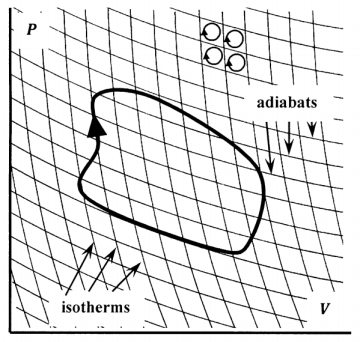
To do so, we introduce an experience-based theorem: The pressure–volume diagram for any reversible system can be tiled by intersecting lines that represent isothermal and adiabatic paths. These lines can be packed as densely as we please, so that the tiling of the pressure–volume diagram can be made as closely spaced as we please. The perimeter of any one of the resulting tiles corresponds to a path around a Carnot cycle. Given any arbitrary closed curve on the pressure–volume diagram, we can select a set of tiles that just encloses it. See Figure 4. The perimeter of this set of tiles approximates the path of the arbitrary curve. Since the tiling can be made as fine as we please, the perimeter of the set of tiles can be made to approximate the path of the arbitrary curve as closely as we please.
Suppose that we traverse the perimeter of each of the individual tiles in a clockwise direction, adding up \(q^{rev}/T\) as we go. Segments of these perimeters fall into two groups. One group consists of segments that are on the perimeter of the enclosing set of tiles. The other group consists of segments that are common to two tiles. When we traverse both of these tiles in a clockwise direction, the shared segment is traversed once in one direction and once in the other. When we add up \(q^{rev}/T\) for these two traverses of the same segment, we find that the sum is zero, because we have \(q^{rev}/T\) in one direction and \(-q^{rev}/T\) in the other. This means that the sum of \(q^{rev}/T\) around all of the tiles will just be equal to the sum of \(q^{rev}/T\) around those segments that lie on the perimeter of the enclosing set. That is, we have
\[\sum_{ \begin{array}{c} \mathrm{cycle} \\ \mathrm{perimeter} \end{array}} \frac{q^{rev}}{T}+\sum_{ \begin{array}{c} \mathrm{interior} \\ \mathrm{seqments} \end{array}} \frac{q^{rev}}{T}=\sum_{ \begin{array}{c} \mathrm{all} \\ \mathrm{tiles} \end{array}} \left\{\sum_{ \begin{array}{c} \mathrm{tile} \\ \mathrm{perimeter} \end{array}} \frac{q^{rev}}{T}\right\} \nonumber \]
where \[\sum_{ \begin{array}{c} \mathrm{interior} \\ \mathrm{seqments} \end{array} } \frac{q^{rev}}{T}=0 \nonumber \]
because each interior segment is traversed twice, and the two contributions cancel exactly.
This set of tiles has another important property. Since each individual tile represents a reversible Carnot cycle, we know that
\[\sum_{ \begin{array}{c} \mathrm{tile} \\ \mathrm{perimeter} \end{array} }{\frac{q^{rev}}{T}}=0 \nonumber \]
around each individual tile. Since the sum around each tile is zero, the sum of all these sums is zero. It follows that the sum of \({q^{rev}}/{T}\) around the perimeter of the enclosing set is zero:
\[\sum_{ \begin{array}{c} \mathrm{cycle} \\ \mathrm{perimeter} \end{array} }{\frac{q^{rev}}{T}}=0 \nonumber \]
By tiling the pressure–volume plane as densely as necessary, we can make the perimeter of the enclosing set as close as we like to any closed curve. The heat increments become arbitrarily small, and
\[\mathop{\mathrm{lim}}_{q^{rev}\to {dq}^{rev}} \left[\sum_{ \begin{array}{c} cycle \\ perimeter \end{array} } \frac{q^{rev}}{T}\right]\ =\oint{\frac{dq^{rev}}{T}}=0 \nonumber \] For any reversible engine producing pressure–volume work, we have \(\oint{dS=0}\) around any cycle.
We can extend this analysis to reach the same conclusion for a reversible engine that produces any form of work. To see this, let us consider the tiling theorem more carefully. When we say that the adiabats and isotherms tile the pressure–volume plane, we mean that each point in the pressure–volume plane is intersected by one and only one adiabat and by one and only one isotherm. When only pressure–volume work is possible, every point in the pressure–volume plane represents a unique state of the system. Therefore, the tiling theorem asserts that every state of the variable-pressure system can be reached along one and only one adiabat and one and only one isotherm.
From experience, we infer that this statement remains true for any form of work. That is, every state of any reversible system can be reached by one and only one isotherm and by one and only one adiabat when any form of work is done. If more than one form of work is possible, there is an adiabat for each form of work. If changing \({\theta }_1\) and changing \({\theta }_2\) change the energy of the system, the effects on the energy of the system are not necessarily the same. In general, \({\mathit{\Phi}}_1\) is not the same as \({\mathit{\Phi}}_2\), where
\[{\mathit{\Phi}}_i={\left(\frac{\partial E}{\partial {\theta }_i}\right)}_{V,{\theta }_{m\neq i}} \nonumber \]
From §3, we know that a reversible Carnot engine doing any form of work can be matched with a reversible ideal-gas Carnot engine in such a way that the engines complete the successive isothermal and adiabatic steps in parallel. At each step, each engine experiences the same heat, work, energy, and entropy changes as the other. Just as we can plot the reversible ideal-gas Carnot cycle as a closed path in pressure–volume space, we can plot a Carnot cycle producing any other form of work as a closed path with successive isothermal and adiabatic steps in \({\mathit{\Phi}}_i{--\theta }_i\) space. Just as any closed path in pressure–volume space can be tiled (or built up from) arbitrarily small reversible Carnot cycles, so any closed path in \({\mathit{\Phi}}_i{--\theta }_i\) space can be tiled by such cycles. Therefore, the argument we use to show that \(\oint{dS=0}\) for any closed reversible cycle in pressure–volume space applies equally well to a closed reversible cycle in which heat is used to produce any other form of work.