7.9: Measuring Heat

As the idea of heat as a form of transferring energy was first being developed, a unit amount of heat was taken to be the amount that was needed to increase the temperature of a reference material by one degree. Water was the reference material of choice, and the calorie was defined as the quantity of heat that raised the temperature of one gram of water one degree kelvin. The amount of heat exchanged by a known amount of water could then be calculated from the amount by which the temperature of the water changed. If, for example, introducing 63.55 g (1 mole) of copper metal, initially at 274.0 K, into 100 g of water, initially at 373.0 K, resulted in thermal equilibrium at 288.5 K, the water surrendered

\[\mathrm{100\ \ g}\ \times \mathrm{1\ cal\ }{\mathrm{g}}^{\mathrm{-1}}\mathrm{\ }{\mathrm{K}}^{\mathrm{-1}}\times 84.5\ \mathrm{K}=8450\mathrm{\ cal} \nonumber \]

This amount of heat was taken up by the copper, so that 0.092 cal was required to increase the temperature of one gram of copper by one degree K. Given this information, the amount of heat gained or lost by a known mass of copper in any subsequent experiment can be calculated from the change in its temperature.

Joule developed the idea that mechanical work can be converted entirely into heat. The quantity of heat that could be produced from one unit of mechanical work was called the mechanical equivalent of heat. Today we define the unit of heat in mechanical units. That is, we define the unit of energy, the joule (\(\mathrm{J}\)), in terms of the mechanical units mass (\(\mathrm{kg}\)), distance (\(\mathrm{m}\)), and time (\(\mathrm{s}\)). One joule is one newton-meter or one \(\mathrm{kg\ }{\mathrm{m}}^{\mathrm{2}}\mathrm{\ }{\mathrm{s}}^{\mathrm{-2}}\). One calorie is now defined as \(\boldsymbol{\mathrm{4}}.\boldsymbol{\mathrm{184}}\boldsymbol{\mathrm{\ }}\mathrm{J}\), exactly. This definition assumes that heat and work are both forms of energy. This assumption is an intrinsic element of the first law of thermodynamics. This aspect of the first law is, of course, just a restatement of Joule’s original idea.

When we want to measure the heat added to a system, measuring the temperature increase that occurs is often the most convenient method. If we know the temperature increase in the system, and we know the temperature increase that accompanies the addition of one unit of heat, we can calculate the heat input to the system. Evidently, it is useful to know how much the temperature increases when one unit of heat is added to various substances. Let us consider a general procedure for accumulating such information.

Figure 5. Heat capacity is the slope of \(q\) versus \(T\).

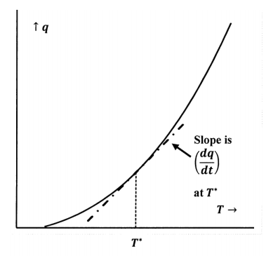
First, we need to choose some standard amount of the substance in question. After all, if we double the amount, it takes twice as much heat to effect the same temperature change. One mole is a natural choice for this standard amount. If we add small increments of heat to one mole of a pure substance, we can measure the temperature after each addition and plot heat versus temperature. Figure 5 shows such a plot. (In experiments like this, it is often convenient to introduce the heat by passing a known electrical current, \(I\), through a known resistance, \(R\), immersed in the substance. The rate at which heat is produced is \(I^{\mathrm{2}}R\). Except for the usually negligible amount that goes into warming the resistor, all of it is transferred to the substance.) At any particular temperature, the slope of the graph is the increment of heat input divided by the incremental temperature increase. This slope is so useful, it is given a name; it is the molar heat capacity of the substance, \(C\). Since this slope is also the derivative of the \(q\)-versus-\(T\) curve, we have

\[C=\frac{dq}{dT} \nonumber \]

The temperature increase accompanying a given heat input varies with the particular conditions under which the experiment is done. In particular, the temperature increase will be less if some of the added heat is converted to work, as is the case if the volume of the system increases. If the volume increases, the system does work on the surroundings. For a given \(q\), \(\Delta T\) will be less when the system is allowed to expand, which means that \({q}/{\Delta T}\) will be greater. Heat capacity measurements are most conveniently done with the system at a constant pressure. However, the heat capacity at constant volume plays an important role in our theoretical development. The heat capacity is denoted \(C_P\) when the pressure is constant and \(C_V\) when the volume is constant. We have the important definitions

\[C_P={\left(\frac{\partial q}{\partial T}\right)}_P \nonumber \] and \[C_V={\left(\frac{\partial q}{\partial T}\right)}_V \nonumber \]

Since no pressure–volume work can be done when the volume is constant, less heat is required to effect a given temperature change, and we have \(C_P>C_V\), as a general result. (In §14, we consider this point further.) If the system contains a gas, the effect of the volume increase can be substantial. For a monatomic ideal gas, the temperature increase at constant pressure is only \(\mathrm{60\%}\) of the temperature increase at constant volume for the same input of heat.