
7.4: Exact Differentials and State Functions
- Page ID
- 151693

\( \newcommand{\vecs}[1]{\overset { \scriptstyle \rightharpoonup} {\mathbf{#1}} } \)
\( \newcommand{\vecd}[1]{\overset{-\!-\!\rightharpoonup}{\vphantom{a}\smash {#1}}} \)
\( \newcommand{\id}{\mathrm{id}}\) \( \newcommand{\Span}{\mathrm{span}}\)
( \newcommand{\kernel}{\mathrm{null}\,}\) \( \newcommand{\range}{\mathrm{range}\,}\)
\( \newcommand{\RealPart}{\mathrm{Re}}\) \( \newcommand{\ImaginaryPart}{\mathrm{Im}}\)
\( \newcommand{\Argument}{\mathrm{Arg}}\) \( \newcommand{\norm}[1]{\| #1 \|}\)
\( \newcommand{\inner}[2]{\langle #1, #2 \rangle}\)
\( \newcommand{\Span}{\mathrm{span}}\)
\( \newcommand{\id}{\mathrm{id}}\)
\( \newcommand{\Span}{\mathrm{span}}\)
\( \newcommand{\kernel}{\mathrm{null}\,}\)
\( \newcommand{\range}{\mathrm{range}\,}\)
\( \newcommand{\RealPart}{\mathrm{Re}}\)
\( \newcommand{\ImaginaryPart}{\mathrm{Im}}\)
\( \newcommand{\Argument}{\mathrm{Arg}}\)
\( \newcommand{\norm}[1]{\| #1 \|}\)
\( \newcommand{\inner}[2]{\langle #1, #2 \rangle}\)
\( \newcommand{\Span}{\mathrm{span}}\) \( \newcommand{\AA}{\unicode[.8,0]{x212B}}\)
\( \newcommand{\vectorA}[1]{\vec{#1}} % arrow\)
\( \newcommand{\vectorAt}[1]{\vec{\text{#1}}} % arrow\)
\( \newcommand{\vectorB}[1]{\overset { \scriptstyle \rightharpoonup} {\mathbf{#1}} } \)
\( \newcommand{\vectorC}[1]{\textbf{#1}} \)
\( \newcommand{\vectorD}[1]{\overrightarrow{#1}} \)
\( \newcommand{\vectorDt}[1]{\overrightarrow{\text{#1}}} \)
\( \newcommand{\vectE}[1]{\overset{-\!-\!\rightharpoonup}{\vphantom{a}\smash{\mathbf {#1}}}} \)
\( \newcommand{\vecs}[1]{\overset { \scriptstyle \rightharpoonup} {\mathbf{#1}} } \)
\( \newcommand{\vecd}[1]{\overset{-\!-\!\rightharpoonup}{\vphantom{a}\smash {#1}}} \)
\(\newcommand{\avec}{\mathbf a}\) \(\newcommand{\bvec}{\mathbf b}\) \(\newcommand{\cvec}{\mathbf c}\) \(\newcommand{\dvec}{\mathbf d}\) \(\newcommand{\dtil}{\widetilde{\mathbf d}}\) \(\newcommand{\evec}{\mathbf e}\) \(\newcommand{\fvec}{\mathbf f}\) \(\newcommand{\nvec}{\mathbf n}\) \(\newcommand{\pvec}{\mathbf p}\) \(\newcommand{\qvec}{\mathbf q}\) \(\newcommand{\svec}{\mathbf s}\) \(\newcommand{\tvec}{\mathbf t}\) \(\newcommand{\uvec}{\mathbf u}\) \(\newcommand{\vvec}{\mathbf v}\) \(\newcommand{\wvec}{\mathbf w}\) \(\newcommand{\xvec}{\mathbf x}\) \(\newcommand{\yvec}{\mathbf y}\) \(\newcommand{\zvec}{\mathbf z}\) \(\newcommand{\rvec}{\mathbf r}\) \(\newcommand{\mvec}{\mathbf m}\) \(\newcommand{\zerovec}{\mathbf 0}\) \(\newcommand{\onevec}{\mathbf 1}\) \(\newcommand{\real}{\mathbb R}\) \(\newcommand{\twovec}[2]{\left[\begin{array}{r}#1 \\ #2 \end{array}\right]}\) \(\newcommand{\ctwovec}[2]{\left[\begin{array}{c}#1 \\ #2 \end{array}\right]}\) \(\newcommand{\threevec}[3]{\left[\begin{array}{r}#1 \\ #2 \\ #3 \end{array}\right]}\) \(\newcommand{\cthreevec}[3]{\left[\begin{array}{c}#1 \\ #2 \\ #3 \end{array}\right]}\) \(\newcommand{\fourvec}[4]{\left[\begin{array}{r}#1 \\ #2 \\ #3 \\ #4 \end{array}\right]}\) \(\newcommand{\cfourvec}[4]{\left[\begin{array}{c}#1 \\ #2 \\ #3 \\ #4 \end{array}\right]}\) \(\newcommand{\fivevec}[5]{\left[\begin{array}{r}#1 \\ #2 \\ #3 \\ #4 \\ #5 \\ \end{array}\right]}\) \(\newcommand{\cfivevec}[5]{\left[\begin{array}{c}#1 \\ #2 \\ #3 \\ #4 \\ #5 \\ \end{array}\right]}\) \(\newcommand{\mattwo}[4]{\left[\begin{array}{rr}#1 \amp #2 \\ #3 \amp #4 \\ \end{array}\right]}\) \(\newcommand{\laspan}[1]{\text{Span}\{#1\}}\) \(\newcommand{\bcal}{\cal B}\) \(\newcommand{\ccal}{\cal C}\) \(\newcommand{\scal}{\cal S}\) \(\newcommand{\wcal}{\cal W}\) \(\newcommand{\ecal}{\cal E}\) \(\newcommand{\coords}[2]{\left\{#1\right\}_{#2}}\) \(\newcommand{\gray}[1]{\color{gray}{#1}}\) \(\newcommand{\lgray}[1]{\color{lightgray}{#1}}\) \(\newcommand{\rank}{\operatorname{rank}}\) \(\newcommand{\row}{\text{Row}}\) \(\newcommand{\col}{\text{Col}}\) \(\renewcommand{\row}{\text{Row}}\) \(\newcommand{\nul}{\text{Nul}}\) \(\newcommand{\var}{\text{Var}}\) \(\newcommand{\corr}{\text{corr}}\) \(\newcommand{\len}[1]{\left|#1\right|}\) \(\newcommand{\bbar}{\overline{\bvec}}\) \(\newcommand{\bhat}{\widehat{\bvec}}\) \(\newcommand{\bperp}{\bvec^\perp}\) \(\newcommand{\xhat}{\widehat{\xvec}}\) \(\newcommand{\vhat}{\widehat{\vvec}}\) \(\newcommand{\uhat}{\widehat{\uvec}}\) \(\newcommand{\what}{\widehat{\wvec}}\) \(\newcommand{\Sighat}{\widehat{\Sigma}}\) \(\newcommand{\lt}{<}\) \(\newcommand{\gt}{>}\) \(\newcommand{\amp}{&}\) \(\definecolor{fillinmathshade}{gray}{0.9}\)Now, let us consider the general case of a continuous function \(f\left(x,y\right)\), for which the exact differential is
\[df=f_x\left(x,y\right)dx+f_y\left(x,y\right)dy. \nonumber \]
We want to integrate the exact differential over very short paths like paths a and b in Section 7.3. Let us evaluate the integral between \(\left(x_0,y_0\right)\) and \(\left(x_0+\Delta x,y_0+\Delta y\right)\) over the paths a* and b* sketched in Figure 3.
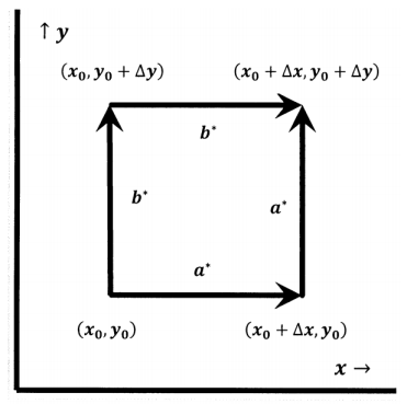
- Path a* has two linear segments. The first segment is the portion of the line \({y=y}_0\) as \(x\) goes from \(x_0\) to \(x_0+\Delta x\). Along the first segment \(\Delta y=0\). The second segment is the portion of the line \({x=x}_0+\Delta x\) as \(y\) goes from \(y_0\) to \(y_0+\Delta y\). Along the second segment, \(\Delta x=0\).
- Path b* has two linear segments also. The first segment is the portion of the line \(x=x_0\) as \(y\) goes from \(y_0\) to \(y_0+\Delta y\). Along the first segment, \(\Delta x=0\). The second segment is the portion of the line \({y=y}_0+\Delta y\) as \(x\) goes from \(x_0\) to \(x_0+\Delta x\). Along the second segment, \(\Delta y=0\).
Along path a*, we have
\[{\Delta }_{a^*}f=f_x\left(x_0,y_0\right)\Delta x+f_y\left(x_0+\Delta x,y_0\right)\Delta y\nonumber \]
Along path b*,
\[{\Delta }_{b^*}f=f_x\left(x_0,y_0+\Delta y\right)\Delta x+f_y\left(x_0,y_0\right)\Delta y\nonumber \]
In the limit as \(\Delta x\) and \(\Delta y\) become arbitrarily small, we must have \({\Delta }_{a^*}f={\Delta }_{b^*}f\), so that
\[f_x\left(x_0,y_0\right)\Delta x+f_y\left(x_0+\Delta x,y_0\right)\Delta y=f_x\left(x_0,y_0+\Delta y\right)\Delta x+f_y\left(x_0,y_0\right)\Delta y\nonumber \]
Rearranging this equation so that terms in \(f_x\) are on one side and terms in \(f_y\) are on the other side, dividing both sides by \(\Delta x\Delta y\), and taking the limit as \(\Delta x\to 0\) and \(\Delta y\to 0\), we have
\[{\mathop{\mathrm{lim}}_{\Delta x\to 0} \left[\frac{f_y\left(x_0+\Delta x,y_0\right)-f_y\left(x_0,y_0\right)}{\Delta x}\right]\ }={\mathop{\mathrm{lim}}_{\Delta y\to 0} \left[\frac{f_x\left(x_0,y_0+\Delta y\right)-f_x\left(x_0,y_0\right)}{\Delta y}\right]\ }\nonumber \]
These limits are the partial derivative of \(f_y\left(x_0,y_0\right)\) with respect to \(x\) and of \(f_x\left(x_0,y_0\right)\) with respect to \(y\). That is
\[{\left[{\frac{\partial }{\partial x}f}_y\left(x_0,y_0\right)\right]}_y={\left[\frac{\partial }{\partial x}\left(\frac{\partial f\left(x_0,y_0\right)}{\partial y}\right)\right]}_y=\frac{{\partial }^2f\left(x_0,y_0\right)}{\partial y\partial x}\nonumber \] and \[{\left[{\frac{\partial }{\partial y}f}_x\left(x_0,y_0\right)\right]}_x={\left[\frac{\partial }{\partial y}\left(\frac{\partial f\left(x_0,y_0\right)}{\partial x}\right)\right]}_x=\frac{{\partial }^2f\left(x_0,y_0\right)}{\partial x\partial y}\nonumber \]
This shows that, if \(f\left(x,y\right)\) is a continuous function of \(x\) and \(y\) whose partial derivatives exist, then
\[\frac{{\partial }^2f\left(x_0,y_0\right)}{\partial y\partial x}=\frac{{\partial }^2f\left(x_0,y_0\right)}{\partial x\partial y}\nonumber \]
The mixed second partial derivative of \(f\left(x,y\right)\) is independent of the order of differentiation. We also write these second partial derivatives as \(f_{xy}\left(x_0,y_0\right)\) and \(f_{yx}\left(x_0,y_0\right)\).
To summarize these points, if \(f\left(x,y\right)\) is a continuous function of \(x\) and \(y\), all of the following are true:
- \(f\left(x,y\right)\) represents a surface in a three-dimensional space.
- \(f\left(x,y\right)\) is a state function.
- The total differential is \[df={\left({\partial f}/{\partial x}\right)}_ydx+{\left({\partial f}/{\partial y}\right)}_xdy.\nonumber \]
- The total differential is exact.
- The line integral of \(df\) between two points is independent of the path of integration.
- The line integral of \(df\) around any closed path is zero: \(\oint{df=0}\).
- The mixed second-partial derivatives are equal; that is, \[\frac{{\partial }^2f}{\partial y\partial x}=\frac{{\partial }^2f}{\partial x\partial y}\nonumber \]