
4.8: Statistics for Molecular Speeds
- Page ID
- 151991

\( \newcommand{\vecs}[1]{\overset { \scriptstyle \rightharpoonup} {\mathbf{#1}} } \)
\( \newcommand{\vecd}[1]{\overset{-\!-\!\rightharpoonup}{\vphantom{a}\smash {#1}}} \)
\( \newcommand{\id}{\mathrm{id}}\) \( \newcommand{\Span}{\mathrm{span}}\)
( \newcommand{\kernel}{\mathrm{null}\,}\) \( \newcommand{\range}{\mathrm{range}\,}\)
\( \newcommand{\RealPart}{\mathrm{Re}}\) \( \newcommand{\ImaginaryPart}{\mathrm{Im}}\)
\( \newcommand{\Argument}{\mathrm{Arg}}\) \( \newcommand{\norm}[1]{\| #1 \|}\)
\( \newcommand{\inner}[2]{\langle #1, #2 \rangle}\)
\( \newcommand{\Span}{\mathrm{span}}\)
\( \newcommand{\id}{\mathrm{id}}\)
\( \newcommand{\Span}{\mathrm{span}}\)
\( \newcommand{\kernel}{\mathrm{null}\,}\)
\( \newcommand{\range}{\mathrm{range}\,}\)
\( \newcommand{\RealPart}{\mathrm{Re}}\)
\( \newcommand{\ImaginaryPart}{\mathrm{Im}}\)
\( \newcommand{\Argument}{\mathrm{Arg}}\)
\( \newcommand{\norm}[1]{\| #1 \|}\)
\( \newcommand{\inner}[2]{\langle #1, #2 \rangle}\)
\( \newcommand{\Span}{\mathrm{span}}\) \( \newcommand{\AA}{\unicode[.8,0]{x212B}}\)
\( \newcommand{\vectorA}[1]{\vec{#1}} % arrow\)
\( \newcommand{\vectorAt}[1]{\vec{\text{#1}}} % arrow\)
\( \newcommand{\vectorB}[1]{\overset { \scriptstyle \rightharpoonup} {\mathbf{#1}} } \)
\( \newcommand{\vectorC}[1]{\textbf{#1}} \)
\( \newcommand{\vectorD}[1]{\overrightarrow{#1}} \)
\( \newcommand{\vectorDt}[1]{\overrightarrow{\text{#1}}} \)
\( \newcommand{\vectE}[1]{\overset{-\!-\!\rightharpoonup}{\vphantom{a}\smash{\mathbf {#1}}}} \)
\( \newcommand{\vecs}[1]{\overset { \scriptstyle \rightharpoonup} {\mathbf{#1}} } \)
\( \newcommand{\vecd}[1]{\overset{-\!-\!\rightharpoonup}{\vphantom{a}\smash {#1}}} \)
\(\newcommand{\avec}{\mathbf a}\) \(\newcommand{\bvec}{\mathbf b}\) \(\newcommand{\cvec}{\mathbf c}\) \(\newcommand{\dvec}{\mathbf d}\) \(\newcommand{\dtil}{\widetilde{\mathbf d}}\) \(\newcommand{\evec}{\mathbf e}\) \(\newcommand{\fvec}{\mathbf f}\) \(\newcommand{\nvec}{\mathbf n}\) \(\newcommand{\pvec}{\mathbf p}\) \(\newcommand{\qvec}{\mathbf q}\) \(\newcommand{\svec}{\mathbf s}\) \(\newcommand{\tvec}{\mathbf t}\) \(\newcommand{\uvec}{\mathbf u}\) \(\newcommand{\vvec}{\mathbf v}\) \(\newcommand{\wvec}{\mathbf w}\) \(\newcommand{\xvec}{\mathbf x}\) \(\newcommand{\yvec}{\mathbf y}\) \(\newcommand{\zvec}{\mathbf z}\) \(\newcommand{\rvec}{\mathbf r}\) \(\newcommand{\mvec}{\mathbf m}\) \(\newcommand{\zerovec}{\mathbf 0}\) \(\newcommand{\onevec}{\mathbf 1}\) \(\newcommand{\real}{\mathbb R}\) \(\newcommand{\twovec}[2]{\left[\begin{array}{r}#1 \\ #2 \end{array}\right]}\) \(\newcommand{\ctwovec}[2]{\left[\begin{array}{c}#1 \\ #2 \end{array}\right]}\) \(\newcommand{\threevec}[3]{\left[\begin{array}{r}#1 \\ #2 \\ #3 \end{array}\right]}\) \(\newcommand{\cthreevec}[3]{\left[\begin{array}{c}#1 \\ #2 \\ #3 \end{array}\right]}\) \(\newcommand{\fourvec}[4]{\left[\begin{array}{r}#1 \\ #2 \\ #3 \\ #4 \end{array}\right]}\) \(\newcommand{\cfourvec}[4]{\left[\begin{array}{c}#1 \\ #2 \\ #3 \\ #4 \end{array}\right]}\) \(\newcommand{\fivevec}[5]{\left[\begin{array}{r}#1 \\ #2 \\ #3 \\ #4 \\ #5 \\ \end{array}\right]}\) \(\newcommand{\cfivevec}[5]{\left[\begin{array}{c}#1 \\ #2 \\ #3 \\ #4 \\ #5 \\ \end{array}\right]}\) \(\newcommand{\mattwo}[4]{\left[\begin{array}{rr}#1 \amp #2 \\ #3 \amp #4 \\ \end{array}\right]}\) \(\newcommand{\laspan}[1]{\text{Span}\{#1\}}\) \(\newcommand{\bcal}{\cal B}\) \(\newcommand{\ccal}{\cal C}\) \(\newcommand{\scal}{\cal S}\) \(\newcommand{\wcal}{\cal W}\) \(\newcommand{\ecal}{\cal E}\) \(\newcommand{\coords}[2]{\left\{#1\right\}_{#2}}\) \(\newcommand{\gray}[1]{\color{gray}{#1}}\) \(\newcommand{\lgray}[1]{\color{lightgray}{#1}}\) \(\newcommand{\rank}{\operatorname{rank}}\) \(\newcommand{\row}{\text{Row}}\) \(\newcommand{\col}{\text{Col}}\) \(\renewcommand{\row}{\text{Row}}\) \(\newcommand{\nul}{\text{Nul}}\) \(\newcommand{\var}{\text{Var}}\) \(\newcommand{\corr}{\text{corr}}\) \(\newcommand{\len}[1]{\left|#1\right|}\) \(\newcommand{\bbar}{\overline{\bvec}}\) \(\newcommand{\bhat}{\widehat{\bvec}}\) \(\newcommand{\bperp}{\bvec^\perp}\) \(\newcommand{\xhat}{\widehat{\xvec}}\) \(\newcommand{\vhat}{\widehat{\vvec}}\) \(\newcommand{\uhat}{\widehat{\uvec}}\) \(\newcommand{\what}{\widehat{\wvec}}\) \(\newcommand{\Sighat}{\widehat{\Sigma}}\) \(\newcommand{\lt}{<}\) \(\newcommand{\gt}{>}\) \(\newcommand{\amp}{&}\) \(\definecolor{fillinmathshade}{gray}{0.9}\)Expected values for several quantities can be calculated from the Maxwell-Boltzmann probability density function. The required definite integrals are tabulated in Appendix D.
The most probable speed, \(v_{mp}\), is the speed at which the Maxwell-Boltzmann equation takes on its maximum value. At this speed, we have
\[ \begin{align*} 0&=\frac{d}{dv}\left(\frac{df\left(v\right)}{dv}\right)=\frac{d}{dv}\left[4\pi {\left(\frac{m}{2\pi kT}\right)}^{3/2}v^2\exp\left(\frac{-mv^2}{2kT}\right)\right] \\[4pt] &=\left[4\pi {\left(\frac{m}{2\pi kT}\right)}^{3/2}\exp\left(\frac{-mv^2}{2kT}\right)\right]\left[2v-\frac{mv^3}{kT}\right] \end{align*} \nonumber \]
from which
\[v_{mp}=\sqrt{\frac{2kT}{m}}\approx 1.414\sqrt{\frac{kT}{m}} \nonumber \]
The average speed, \(\overline{v}\) or \(\left\langle v\right\rangle\), is the expected value of the scalar velocity (\(g\left(v\right)=v\)). We find
\[\overline{v}=\left\langle v\right\rangle =\int^{\infty }_0{4\pi {\left(\frac{m}{2\pi kT}\right)}^{3/2}v^3exp\left(\frac{-mv^2}{2kT}\right)}dv=\sqrt{\frac{8kT}{\pi m}}\approx 1.596\sqrt{\frac{kT}{m}} \nonumber \]
The mean-square speed, \(\overline{v^2}\) or \(\left\langle v^2\right\rangle\), is the expected value of the velocity squared (\(g\left(v\right)=v^2\)):
\[\overline{v^2}=\left\langle v^2\right\rangle =\int^{\infty }_0{4\pi {\left(\frac{m}{2\pi kT}\right)}^{3/2}v^4exp\left(\frac{-mv^2}{2kT}\right)}dv=\frac{3kT}{m} \nonumber \]
and the root mean-square speed, \(v_{rms}\), is
\[v_{rms}=\sqrt{\left\langle v^2\right\rangle }=\sqrt{\frac{3kT}{m}}\approx 1.732\sqrt{\frac{kT}{m}} \nonumber \]
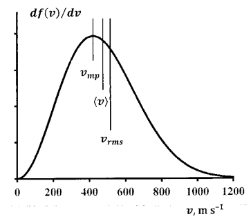
Figure 6 shows the velocity distribution 300 K for nitrogen molecules at 300 K.
Solution
Finally, let us find the variance of the velocity; that is, the expected value of \(\left(v-\left\langle v\right\rangle \right)^2\):
\({\text { variance }(v)=\sigma_{v}^{2}} \)
\[\begin{align*} &=\int_{0}^{\infty}(v-\langle v\rangle)^{2}\left(\frac{d f(v)}{d v}\right) d v \\ &=\int_{0}^{\infty} v^{2}\left(\frac{d f}{d v}\right) d v-2\langle v\rangle \int_{0}^{\infty} v\left(\frac{d f}{d v}\right) d v+\langle v\rangle^{2} \int_{0}^{\infty}\left(\frac{d f}{d v}\right) \\ &=\left\langle v^{2}\right\rangle- 2\langle v\rangle\langle v\rangle+\langle v\rangle^{2} \\ &=\left\langle v^{2}\right\rangle-\langle v\rangle^{2} \end{align*} \nonumber \]
For \(N_2\) at \(300\) K, we calculate:
\[v_{mp}\ =422\ \mathrm{m\ }{\mathrm{s}}^{\mathrm{-1}} \nonumber \]
\[\left\langle v\right\rangle =\overline{v}=476\ \mathrm{m\ }{\mathrm{s}}^{\mathrm{-1}} \nonumber \]
\[v_{rms}=517\ \mathrm{m\ }{\mathrm{s}}^{\mathrm{-1}} \nonumber \]
\[ \text{Variance} \left(v\right)=\sigma^2_v=40.23\times {10}^{-3}\ \mathrm{m\ }{\mathrm{s}}^{\mathrm{-1}} \nonumber \]
\[\sigma_v=201\ \mathrm{m\ }{\mathrm{s}}^{\mathrm{-1}} \nonumber \]