
3.10: Statistics - the Mean and the Variance of a Distribution
- Page ID
- 151671

\( \newcommand{\vecs}[1]{\overset { \scriptstyle \rightharpoonup} {\mathbf{#1}} } \)
\( \newcommand{\vecd}[1]{\overset{-\!-\!\rightharpoonup}{\vphantom{a}\smash {#1}}} \)
\( \newcommand{\id}{\mathrm{id}}\) \( \newcommand{\Span}{\mathrm{span}}\)
( \newcommand{\kernel}{\mathrm{null}\,}\) \( \newcommand{\range}{\mathrm{range}\,}\)
\( \newcommand{\RealPart}{\mathrm{Re}}\) \( \newcommand{\ImaginaryPart}{\mathrm{Im}}\)
\( \newcommand{\Argument}{\mathrm{Arg}}\) \( \newcommand{\norm}[1]{\| #1 \|}\)
\( \newcommand{\inner}[2]{\langle #1, #2 \rangle}\)
\( \newcommand{\Span}{\mathrm{span}}\)
\( \newcommand{\id}{\mathrm{id}}\)
\( \newcommand{\Span}{\mathrm{span}}\)
\( \newcommand{\kernel}{\mathrm{null}\,}\)
\( \newcommand{\range}{\mathrm{range}\,}\)
\( \newcommand{\RealPart}{\mathrm{Re}}\)
\( \newcommand{\ImaginaryPart}{\mathrm{Im}}\)
\( \newcommand{\Argument}{\mathrm{Arg}}\)
\( \newcommand{\norm}[1]{\| #1 \|}\)
\( \newcommand{\inner}[2]{\langle #1, #2 \rangle}\)
\( \newcommand{\Span}{\mathrm{span}}\) \( \newcommand{\AA}{\unicode[.8,0]{x212B}}\)
\( \newcommand{\vectorA}[1]{\vec{#1}} % arrow\)
\( \newcommand{\vectorAt}[1]{\vec{\text{#1}}} % arrow\)
\( \newcommand{\vectorB}[1]{\overset { \scriptstyle \rightharpoonup} {\mathbf{#1}} } \)
\( \newcommand{\vectorC}[1]{\textbf{#1}} \)
\( \newcommand{\vectorD}[1]{\overrightarrow{#1}} \)
\( \newcommand{\vectorDt}[1]{\overrightarrow{\text{#1}}} \)
\( \newcommand{\vectE}[1]{\overset{-\!-\!\rightharpoonup}{\vphantom{a}\smash{\mathbf {#1}}}} \)
\( \newcommand{\vecs}[1]{\overset { \scriptstyle \rightharpoonup} {\mathbf{#1}} } \)
\( \newcommand{\vecd}[1]{\overset{-\!-\!\rightharpoonup}{\vphantom{a}\smash {#1}}} \)
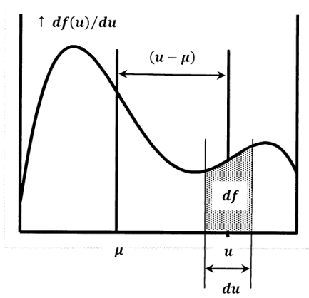
\(\newcommand{\avec}{\mathbf a}\) \(\newcommand{\bvec}{\mathbf b}\) \(\newcommand{\cvec}{\mathbf c}\) \(\newcommand{\dvec}{\mathbf d}\) \(\newcommand{\dtil}{\widetilde{\mathbf d}}\) \(\newcommand{\evec}{\mathbf e}\) \(\newcommand{\fvec}{\mathbf f}\) \(\newcommand{\nvec}{\mathbf n}\) \(\newcommand{\pvec}{\mathbf p}\) \(\newcommand{\qvec}{\mathbf q}\) \(\newcommand{\svec}{\mathbf s}\) \(\newcommand{\tvec}{\mathbf t}\) \(\newcommand{\uvec}{\mathbf u}\) \(\newcommand{\vvec}{\mathbf v}\) \(\newcommand{\wvec}{\mathbf w}\) \(\newcommand{\xvec}{\mathbf x}\) \(\newcommand{\yvec}{\mathbf y}\) \(\newcommand{\zvec}{\mathbf z}\) \(\newcommand{\rvec}{\mathbf r}\) \(\newcommand{\mvec}{\mathbf m}\) \(\newcommand{\zerovec}{\mathbf 0}\) \(\newcommand{\onevec}{\mathbf 1}\) \(\newcommand{\real}{\mathbb R}\) \(\newcommand{\twovec}[2]{\left[\begin{array}{r}#1 \\ #2 \end{array}\right]}\) \(\newcommand{\ctwovec}[2]{\left[\begin{array}{c}#1 \\ #2 \end{array}\right]}\) \(\newcommand{\threevec}[3]{\left[\begin{array}{r}#1 \\ #2 \\ #3 \end{array}\right]}\) \(\newcommand{\cthreevec}[3]{\left[\begin{array}{c}#1 \\ #2 \\ #3 \end{array}\right]}\) \(\newcommand{\fourvec}[4]{\left[\begin{array}{r}#1 \\ #2 \\ #3 \\ #4 \end{array}\right]}\) \(\newcommand{\cfourvec}[4]{\left[\begin{array}{c}#1 \\ #2 \\ #3 \\ #4 \end{array}\right]}\) \(\newcommand{\fivevec}[5]{\left[\begin{array}{r}#1 \\ #2 \\ #3 \\ #4 \\ #5 \\ \end{array}\right]}\) \(\newcommand{\cfivevec}[5]{\left[\begin{array}{c}#1 \\ #2 \\ #3 \\ #4 \\ #5 \\ \end{array}\right]}\) \(\newcommand{\mattwo}[4]{\left[\begin{array}{rr}#1 \amp #2 \\ #3 \amp #4 \\ \end{array}\right]}\) \(\newcommand{\laspan}[1]{\text{Span}\{#1\}}\) \(\newcommand{\bcal}{\cal B}\) \(\newcommand{\ccal}{\cal C}\) \(\newcommand{\scal}{\cal S}\) \(\newcommand{\wcal}{\cal W}\) \(\newcommand{\ecal}{\cal E}\) \(\newcommand{\coords}[2]{\left\{#1\right\}_{#2}}\) \(\newcommand{\gray}[1]{\color{gray}{#1}}\) \(\newcommand{\lgray}[1]{\color{lightgray}{#1}}\) \(\newcommand{\rank}{\operatorname{rank}}\) \(\newcommand{\row}{\text{Row}}\) \(\newcommand{\col}{\text{Col}}\) \(\renewcommand{\row}{\text{Row}}\) \(\newcommand{\nul}{\text{Nul}}\) \(\newcommand{\var}{\text{Var}}\) \(\newcommand{\corr}{\text{corr}}\) \(\newcommand{\len}[1]{\left|#1\right|}\) \(\newcommand{\bbar}{\overline{\bvec}}\) \(\newcommand{\bhat}{\widehat{\bvec}}\) \(\newcommand{\bperp}{\bvec^\perp}\) \(\newcommand{\xhat}{\widehat{\xvec}}\) \(\newcommand{\vhat}{\widehat{\vvec}}\) \(\newcommand{\uhat}{\widehat{\uvec}}\) \(\newcommand{\what}{\widehat{\wvec}}\) \(\newcommand{\Sighat}{\widehat{\Sigma}}\) \(\newcommand{\lt}{<}\) \(\newcommand{\gt}{>}\) \(\newcommand{\amp}{&}\) \(\definecolor{fillinmathshade}{gray}{0.9}\)There are two important statistics associated with any probability distribution, the mean of a distribution and the variance of a distribution. The mean is defined as the expected value of the random variable itself. The Greek letter \(\mu\) is usually used to represent the mean. If \(f\left(u\right)\) is the cumulative probability distribution, the mean is the expected value for \(g\left(u\right)=u\). From our definition of expected value, the mean is
\[\mu =\int^{\infty }_{-\infty }{u\left(\frac{df}{du}\right)du} \nonumber \]
The variance is defined as the expected value of \({\left(u-\mu \right)}^2\). The variance measures how dispersed the data are. If the variance is large, the data are—on average—farther from the mean than they are if the variance is small. The standard deviation is the square root of the variance. The Greek letter \(\sigma\) is usually used to denote the standard deviation. Then, \(\sigma^2\) denotes the variance, and
\[\sigma^2=\int^{\infty }_{-\infty }{{\left(u-\mu \right)}^2\left(\frac{df}{du}\right)du} \nonumber \]
If we have a small number of points from a distribution, we can estimate \(\mu\) and \(\sigma\) by approximating these integrals as sums over the domain of the random variable. To do this, we need to estimate the probability associated with each interval for which we have a sample point. By the argument we make in Section 3.7, the best estimate of this probability is simply \({1}/{N}\), where \(N\) is the number of sample points. We have therefore
\[\mu =\int^{\infty }_{-\infty }{u\left(\frac{df}{du}\right)du\approx \sum^N_1{u_i\left(\frac{1}{N}\right)=\overline{u}}} \nonumber \]
That is, the best estimate we can make of the mean from \(N\) data points is \(\overline{u}\), where \(\overline{u}\) is the ordinary arithmetic average. Similarly, the best estimate we can make of the variance is
\[ \sigma^2 = \int_{- \infty}^{ \infty} (u - \mu )^2 \left( \frac{df}{du} \right) du \approx \sum_{i=1}^N (u_i - \mu )^2 \left( \frac{1}{N} \right) \nonumber \]
Now a complication arises in that we usually do not know the value of \(\mu\). The best we can do is to estimate its value as \(\mu \approx \overline{u}\). It turns out that using this approximation in the equation we deduce for the variance gives an estimate of the variance that is too small. A more detailed argument (see Section 3.14) shows that, if we use \(\overline{u}\) to approximate the mean, the best estimate of \(\sigma^2\), usually denoted \(s^2\), is
\[estimated\ \sigma^2=s^2=\sum^N_{i=1}{{\left(u_i-\overline{u}\right)}^2\left(\frac{1}{N-1}\right)} \nonumber \]
Dividing by \(N-1\), rather than \(N\), compensates exactly for the error introduced by using \(\overline{u}\) rather than \(\mu\).
The mean is analogous to a center of mass. The variance is analogous to a moment of inertia. For this reason, the variance is also called the second moment about the mean. To show these analogies, let us imagine that we draw the probability density function on a uniformly thick steel plate and then cut along the curve and the \(u\)-axis (Figure \(\PageIndex{1}\)). Let \(M\) be the mass of the cutout piece of plate; \(M\) is the mass below the probability density curve. Let \(dA\) and \(dm\) be the increments of area and mass in the thin slice of the cutout that lies above a small increment, \(du\), of \(u\). Let \(\rho\) be the density of the plate, expressed as mass per unit area. Since the plate is uniform, \(\rho\) is constant. We have \(dA=\left({df}/{du}\right)du\) and \(dm=\rho dA\) so that
\[dm=\rho \left(\frac{df}{du}\right)du \nonumber \]
The mean of the distribution corresponds to a vertical line on this cutout at \(u=\mu\). If the cutout is supported on a knife-edge along the line \(u=\mu\), gravity induces no torque; the cutout is balanced. Since the torque is zero, we have
\[0=\int^M_{m=0}{\left(u-\mu \right)dm=\int^{\infty }_{-\infty }{\left(u-\mu \right)\rho \left(\frac{df}{du}\right)du}} \nonumber \]
Since \(\mu\) is a constant property of the cut-out, it follows that
\[\mu =\int^{\infty }_{-\infty }{u\left(\frac{df}{du}\right)}du \nonumber \]
The cutout’s moment of inertia about the line \(u=\mu\) is
\[\begin{aligned} I & =\int^M_{m=0}{{\left(u-\mu \right)}^2dm} \\ ~ & =\int^{\infty }_{-\infty }{{\left(u-\mu \right)}^2\rho \left(\frac{df}{du}\right)du} \\ ~ & =\rho \sigma^2 \end{aligned} \nonumber \]
The moment of inertia about the line \(u-\mu\) is simply the mass per unit area, \(\rho\), times the variance of the distribution. If we let \(\rho =1\), we have \(I=\sigma^2\).
We define the mean of \(f\left(u\right)\) as the expected value of \(u\). It is the value of \(u\) we should “expect” to get the next time we sample the distribution. Alternatively, we can say that the mean is the best prediction we can make about the value of a future sample from the distribution. If we know \(\mu\), the best prediction we can make is \(u_{predicted}=\mu\). If we have only the estimated mean, \(\overline{u}\), then \(\overline{u}\) is the best prediction we can make. Choosing \(u_{predicted}=\overline{u}\) makes the difference,\(\ \left|u-u_{predicted}\right|\), as small as possible.
These ideas relate to another interpretation of the mean. We saw that the variance is the second moment about the mean. The first moment about the mean is
\[ \begin{aligned} 1^{st}\ moment & =\int^{\infty }_{-\infty }{\left(u-\mu \right)}\left(\frac{df}{du}\right)du \\ ~ & =\int^{\infty }_{-\infty }{u\left(\frac{df}{du}\right)du}-\mu \int^{\infty }_{-\infty }{\left(\frac{df}{du}\right)du} \\ ~ & =\mu -\mu \\ ~ & =0 \end{aligned} \nonumber \]
Since the last two integrals are \(\mu\) and 1, respectively, the first moment about the mean is zero. We could have defined the mean as the value, \(\mu\), for which the first moment of \(u\) about \(\mu\) is zero.
The first moment about the mean is zero. The second moment about the mean is the variance. We can define third, fourth, and higher moments about the mean. Some of these higher moments have useful applications.