15.1: Differential and integrated rate laws

The rate law of a chemical reaction is an equation that links the initial rate with the concentrations (or pressures) of the reactants. Rate laws usually include a constant parameter, \(k\), called the rate coefficient, and several parameters found at the exponent of the concentrations of the reactants, and are called reaction orders. The rate coefficient depends on several conditions, including the reaction type, the temperature, the surface area of an adsorbent, light irradiation, and others. The reaction rate is usually represented with the lowercase letter \(k\), and it should not be confused with the thermodynamic equilibrium constant that is generally designated with the uppercase letter \(K\). Another useful concept in kinetics is the half-life, usually abbreviated with \(t_{1/2}\). The half-life is defined as the time required to reach half of the initial reactant concentration.

A reaction that happens in one single microscopic step is called elementary. Elementary reactions have reaction orders equal to the (integer) stoichiometric coefficients for each reactant. As such, only a limited number of elementary reactions are possible (four types are commonly observed), and they are classified according to their overall reaction order. The global reaction order of a reaction is calculated as the sum of each reactant’s individual orders and is, at most, equal to three. We examine in detail the four most common reaction orders below.

Zeroth-order reaction

For a zeroth-order reaction, the reaction rate is independent of the concentration of a reactant. In other words, if we have a reaction of the type:

\[ \text{A}\longrightarrow\text{products} \nonumber \]

the differential rate law can be written:

\[ - \dfrac{d[\mathrm{A}]}{dt}=k_0 [\mathrm{A}]^0 = k_0, \label{15.1.1} \]

which shows that any change in the concentration of \(\mathrm{A}\) will have no effect on the speed of the reaction. The minus sign at the right-hand-side is required because the rate is always defined as a positive quantity, while the derivative is negative because the concentration of the reactant is diminishing with time. Separating the variables \([\mathrm{A}]\) and \(t\) of Equation \ref{15.1.1} and integrating both sides, we obtain the integrated rate law for a zeroth-order reaction as:

\[ \begin{equation} \begin{aligned} \int_{[\mathrm{A}]_0}^{[A]} d[\mathrm{A}] &= -k_0 \int_{t=0}^{t} dt \\ [\mathrm{A}]-[\mathrm{A}]_0 &= -k_0 t \\ \\ [\mathrm{A}]&=[\mathrm{A}]_0 -k_0 t. \end{aligned} \end{equation} \label{15.1.2} \]

Using the integrated rate law, we notice that the concentration on the reactant diminishes linearly with respect to time. A plot of \([\mathrm{A}]\) as a function of \(t\), therefore, will result in a straight line with an angular coefficient equal to \(-k_0\), as in the plot of Figure \(\PageIndex{1}\).

Figure \(\PageIndex{1}\): Reaction Rate Plot for a Zeroth-Order Reaction.

Eq. (15.1.2) also suggests that the units of the rate coefficient for a zeroth-order reaction are of concentration divided by time, typically \(\dfrac{\mathrm{M}}{\mathrm{s}}\), with \(\mathrm{M}\) being the molar concentration in \(\dfrac{\mathrm{mol}}{\mathrm{L}}\) and \(s\) the time in seconds. The half-life of a zero order reaction can be calculated from Equation \ref{15.1.2}, by replacing \([\mathrm{A}]\) with \(\dfrac{1}{2}[\mathrm{A}]_0\):

\[ \begin{equation} \begin{aligned} \dfrac{1}{2}[\mathrm{A}]_0 &=[\mathrm{A}]_0 -k_0 t_{1/2} \\ t_{1/2} &= \dfrac{[\mathrm{A}]_0}{2k_0}. \end{aligned} \end{equation} \label{15.1.3} \]

Zeroth-order reactions are common in several biochemical processes catalyzed by enzymes, such as the oxidation of ethanol to acetaldehyde in the liver by the alcohol dehydrogenase enzyme, which is zero-order in ethanol.

First-order reaction

A first-order reaction depends on the concentration of only one reactant, and is therefore also called a unimolecular reaction. As for the previous case, if we consider a reaction of the type:

\[ \mathrm{A}\rightarrow \text{products} \nonumber \]

the differential rate law for a first-order reaction is:

\[ - \dfrac{d[\mathrm{A}]}{dt}=k_1 [\mathrm{A}]. \label{15.1.4} \]

Following the usual blueprint of separating the variables, and integrating both sides, we obtain the integrated rate law as:

\[ \begin{equation} \begin{aligned} \int_{[\mathrm{A}]_0}^{[A]} \dfrac{d[\mathrm{A}]}{[\mathrm{A}]} &= -k_1 \int_{t=0}^{t} dt \\ \ln \dfrac{[\mathrm{A}]}{[\mathrm{A}]_0}&=-k_1 t\\ \\ [\mathrm{A}] &= [\mathrm{A}]_0 \exp(-k_1 t). \end{aligned} \end{equation} \label{15.1.5} \]

Using the integrated rate law to plot the concentration of the reactant, \([\mathrm{A}]\), as a function of time, \(t\), we obtain an exponential decay, as in Figure \(\PageIndex{2}\).

Figure \(\PageIndex{2}\): Reaction Rate Plot for a First-Order Reaction.

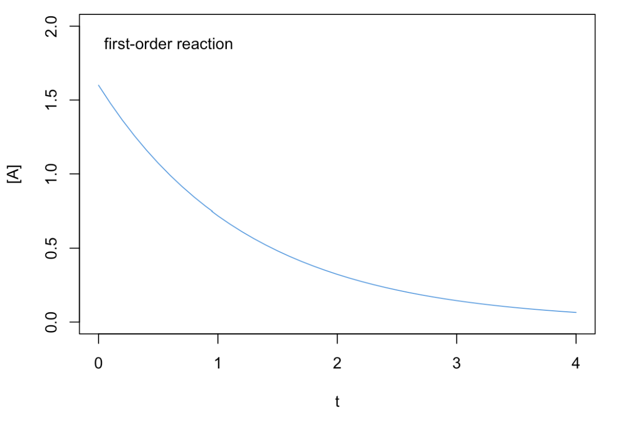
However, if we plot the logarithm of the concentration, \(\ln[\mathrm{A}]\), as a function of time, we obtain a line with angular coefficient \(-k_1\), as in the plot of Figure \(\PageIndex{3}\). From Equation \ref{15.1.5}, we can also obtain the units for the rate coefficient for a first-order reaction, which typically is \(\dfrac{1}{\mathrm{s}}\), independent of concentration. Since the rate coefficient for first-order reactions has units of inverse time, it is sometimes called the frequency rate.

Figure \(\PageIndex{3}\): Linear Plot for a First-Order Reaction. Notice that the Quantity on the y Axes is ln[A].

The half-life of a first-order reaction is:

\[ \begin{equation} \begin{aligned} \ln \dfrac{\dfrac{1}{2}[\mathrm{A}]_0}{[\mathrm{A}]_0}&=-k_1 t_{1/2}\\ t_{1/2} &= \dfrac{\ln 2}{k_1}. \end{aligned} \end{equation} \label{15.1.6} \]

The half-life of a first-order reaction is independent of the initial concentration of the reactant. Therefore, the half-life can be used in place of the rate coefficient to describe the reaction rate. Typical examples of first-order reactions are radioactive decays. For radioactive isotopes, it is common to report their rate of decay in terms of their half-life. For example, the most stable uranium nucleotide, \(^{238}\mathrm{U}\), has a half-life of \(4.468\times 10^9\) years, while the most common fissile isotope of uranium, \(^{235}\mathrm{U}\), has a half-life of \(7.038\times 10^8\) years.\(^1\) Other examples of first-order reactions in chemistry are the class of S_N1 nucleophilic substitution reactions in organic chemistry.

Second-order reaction

A reaction is second-order when the sum of the reaction orders is two. Elementary second-order reactions are also called bimolecular reactions. There are two possibilities, a simple one, where the reaction order of one reagent is two, or a more complicated one, with two reagents having each a reaction order of one.

• For the simple case, we can write the reaction as: \[ 2\mathrm{A}\rightarrow \text{products} \nonumber \] the differential rate law for a first-order reaction is: \[ -\dfrac{d[\mathrm{A}]}{dt}=k_2 [\mathrm{A}]^2. \label{15.1.7} \] Following the same procedure used for the two previous cases, we can obtain the integrated rate law as: \[ \begin{equation} \begin{aligned} \int_{[\mathrm{A}]_0}^{[A]} \dfrac{d[\mathrm{A}]}{[\mathrm{A}]^2} &= -k_2 \int_{t=0}^{t} dt \\ \dfrac{1}{[\mathrm{A}]}-\dfrac{1}{[\mathrm{A}]_0} &= k_2 t\\ \\ \dfrac{1}{[\mathrm{A}]}&=\dfrac{1}{[\mathrm{A}]_0} + k_2 t. \end{aligned} \end{equation} \label{15.1.8} \] As for first-order reactions, the plot of the concentration as a function of time shows a non-linear decay. However, if we plot the inverse of the concentration, \(\dfrac{1}{[\mathrm{A}]}\), as a function of time, \(t\), we obtain a line with angular coefficient \(+k_2\), as in the plot of Figure \(\PageIndex{4}\).

Figure \(\PageIndex{4}\): Linear Plot for a Second-Order Reaction. Notice that the Quantity on the y Axes is 1/[A].

Notice that the line has a positive angular coefficient, in contrast with the previous two cases, for which the angular coefficients were negative. The units of \(k\) for a simple second order reaction are calculated from Equation \ref{15.1.8} and typically are \(\dfrac{1}{\mathrm{M}\cdot \mathrm{s}}\). The half-life of a simple second-order reaction is: \[ \begin{equation} \begin{aligned} \dfrac{1}{\dfrac{1}{2}[\mathrm{A}]_0}-\dfrac{1}{[\mathrm{A}]_0} &= k_2 t_{1/2} \\ t_{1/2} &= \dfrac{1}{k_2 [\mathrm{A}]_0}, \end{aligned} \end{equation} \label{15.1.9} \] which, perhaps not surprisingly, depends on the initial concentration of the reactant, \([\mathrm{A}]_0\). Therefore, if we start with a higher concentration of the reactant, the half-life will be shorter, and the reaction will be faster. An example of simple second-order behavior is the reaction \(\mathrm{NO}_2 + \mathrm{CO} \rightarrow \mathrm{NO} + \mathrm{CO}_2\), which is second-order in \(\mathrm{NO}_2\) and zeroth-order in \(\mathrm{CO}\).

• For the complex second-order case, the reaction is: \[ \mathrm{A}+\mathrm{B}\rightarrow \text{products} \nonumber \] and the differential rate law is: \[ -\dfrac{d[\mathrm{A}]}{dt}=k'_2 [\mathrm{A}][\mathrm{B}]. \label{15.1.10} \] The differential equation in Equation \ref{15.1.10} has two variables, and cannot be solved exactly unless an additional relationship is specified. If we assume that the initial concentration of the two reactants are equal, then \([\mathrm{A}]=[\mathrm{B}]\) at any time \(t\), and Equation \ref{15.1.10} reduces to Equation \ref{15.1.7}. If the concentration of the reactants are different, then the integrated rate law will assume the following shape: \[ \dfrac{\mathrm{[A]}}{\mathrm{[B]}} = \dfrac{\mathrm{[A]_0}}{\mathrm{[B]_0}} \exp \left\{ \left(\mathrm{[A]_0} - \mathrm{[B]_0}\right) k'_2t \right\}. \label{15.1.11} \] The units of \(k\) for a complex second order reaction can be calculated from Equation \ref{15.1.11}, and are the same as those for the simple case, \(\dfrac{1}{\mathrm{M}\cdot \mathrm{s}}\). The half-life of a complex second-order reaction cannot be easily written since two different half-lives could, in principle, be defined for each of the corresponding reactants.

Third and higher orders reaction

Although elementary reactions with order higher than two are possible, they are in practice infrequent, and only very few experimental third-order reactions are observed. Fourth-order or higher have never been observed because the probabilities for a simultaneous interaction between four molecules are essentially zero. Third-order elementary reactions are also called termolelucar reactions. While termolelucar reactions with three identical reactants are possible in principle, there is no known experimental example. Some complex third-order reactions are known, such as:

\[ 2\text{NO}_{(g)}+\text{O}_{2(g)}\longrightarrow 2\text{NO}_{2(g)} \nonumber \]

for which the differential rate law can be written as:

\[ -\dfrac{dP_{\mathrm{O}_2}}{dt}=k_3 P_{\mathrm{NO}}^2 P_{\mathrm{O}_2}. \label{15.1.12} \]

---

1. Notice how large these numbers are for uranium. To put these numbers in perspective, we can compare them with the half-life of the most unstable isotope of plutonium, \(^{241}\mathrm{Pu}\), which is \(t_{1/2}=14.1\) years.︎