13.3: Phase Diagrams of 2-Components/2-Condensed Phases Systems

We now consider equilibria between two condensed phases: liquid/liquid, liquid/solid, and solid/solid. These equilibria usually occur in the low-temperature region of a phase diagram (or high pressure). Three situations are possible, depending on the constituents and concentration of the mixture.

Totally miscible

We have already encountered the situation where the components of a solution mix entirely in the liquid phase. All the diagrams that we’ve discussed up to this point belong to this category.

Totally immiscible

A more complicated case is that for components that do not mix in the liquid phase. The liquid region of the temperature–composition phase diagram for a solution with components that do not mix in the liquid phase below a specific temperature is reported in Figure \(\PageIndex{1}\).

Figure \(\PageIndex{1}\): The Liquid Region of the Temperature–Composition Phase Diagram of Solutions Containing Two Components that are Completely Immiscible in the Liquid Phase.

While the liquid 1+liquid 2 region (white area in Figure \(\PageIndex{1}\)) might seem similar to the liquid region that sits on top of it (blue area in Figure \(\PageIndex{1}\)), it is substantially different in nature. To prove this, we can calculate the degrees of freedom in each region using the Gibbs phase rule. For the liquid region at the top of the diagram, at constant pressure, we have \(f=2-1+1=2\). In other words, the temperature and the composition are independent, and their values can be changed regardless of each other. In the liquid 1+liquid 2 at the bottom, however, we have \(f=2-2+1=1\), which means that only one variable is independent of the others. The white region in Figure \(\PageIndex{1}\) is a 2-phase region, and it behaves similarly to the other 2-phases regions that we encountered before, such as the inner portion of the lens in Figure 13.1.4. In other words, since the two components are entirely immiscible, once we set the temperature at a value below the immiscibility line, the concentration of the two liquids will be determined by tracing a horizontal line and by reading the concentrations on the left and right of the diagram (corresponding to 100% \(\mathrm{A}\) and 100% \(\mathrm{B}\), respectively).

Partially miscible

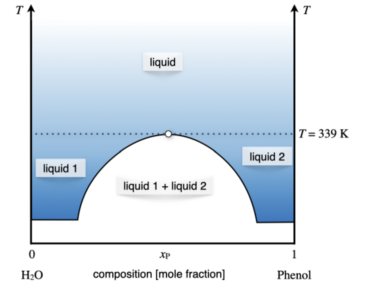
The third and final case is undoubtedly the most interesting since several behaviors are possible. In fact, there might be components that are partially miscible at low temperatures but totally miscible at higher temperatures, for which the diagram will assume the general shape depicted in Figure \(\PageIndex{2}\). A typical example of this behavior is the mixture between water and phenol, whose liquids are completely miscible at \(T>66\;^\circ \text{C}\), and only partially miscible below this temperature. The composition of the 2-phases region (white area in Figure \(\PageIndex{2}\)) is determined by tracing a horizontal line and reading the mole fraction on the line that delimits the area, as for the previous case.\(^1\)

Figure \(\PageIndex{2}\): The Liquid Region of the Temperature–Composition Phase Diagram of Solutions Containing Two Components that are Partially Immiscible at Low Temperature in the Liquid Phase, but Completely Miscible at High Temperatures

On the opposite side of the spectrum, the diagram for a mixture whose components are partially miscible at high temperature, but completely miscible at lower temperatures is depicted in Figure \(\PageIndex{3}\). A typical example of this behavior is the mixture between water and triethylamine, whose liquids are completely miscible at \(T<18.5\;^\circ \text{C}\), and only partially miscible above this temperature.

Figure \(\PageIndex{3}\): The Liquid Region of the Temperature–Composition Phase Diagram of Solutions Containing Two Components that are Partially Immiscible at High Temperature in the Liquid Phase, but Completely Miscible at Low Temperatures.

Finally, both situations described above are possible simultaneously. For some particular solutions, there exists a range of temperature where the two components are only partially miscible. A typical example of this behavior is given by the water/nicotine mixture, whose liquids are completely miscible at \(T>210\;^\circ \text{C}\) and \(T<61\;^\circ \text{C}\), but only partially miscible in between these two temperatures, as in the diagram of Figure \(\PageIndex{4}\).

Figure \(\PageIndex{4}\) : The Liquid Region of the Temperature–Composition Phase Diagram of Solutions Containing Two Components that are Partially Immiscible Only Between Two Temperatures.

Eutectic systems

For some particular mixture, the temperature of partial miscibility in the liquid/liquid region might be close to the azeotrope temperature. In some cases, these two regions might even overlap. These characteristic behaviors are reported in Figure \(\PageIndex{5}\).

Figure \(\PageIndex{5}\): Interaction Between the Liquid/Gas and Liquid/Liquid Equilibria.

When the azeotrope and partially miscibility temperature overlap, the system forms what is known as an eutectic. Eutectic diagrams are possible at the liquid/gas equilibrium. Still, they are widespread at the liquid/solid equilibrium, where two components are completely miscible in the liquid phase, but only partially miscible in the solid phase. Eutectics with completely immiscible components in the solid phase are also very common, as the diagram reported in Figure \(\PageIndex{6}\).

Figure \(\PageIndex{6}\): Typical Eutectic System with Components that are Completely Miscible in the Liquid Phase and Completely Immiscible in the Solid Phase.​​​​​

---

1. The only noticeable difference, in this case, is that the two concentrations will be different than 0 and 100% since the component mix partially.