
11.1: The Ideal Gas Equation
- Page ID
- 414078

\( \newcommand{\vecs}[1]{\overset { \scriptstyle \rightharpoonup} {\mathbf{#1}} } \)
\( \newcommand{\vecd}[1]{\overset{-\!-\!\rightharpoonup}{\vphantom{a}\smash {#1}}} \)
\( \newcommand{\id}{\mathrm{id}}\) \( \newcommand{\Span}{\mathrm{span}}\)
( \newcommand{\kernel}{\mathrm{null}\,}\) \( \newcommand{\range}{\mathrm{range}\,}\)
\( \newcommand{\RealPart}{\mathrm{Re}}\) \( \newcommand{\ImaginaryPart}{\mathrm{Im}}\)
\( \newcommand{\Argument}{\mathrm{Arg}}\) \( \newcommand{\norm}[1]{\| #1 \|}\)
\( \newcommand{\inner}[2]{\langle #1, #2 \rangle}\)
\( \newcommand{\Span}{\mathrm{span}}\)
\( \newcommand{\id}{\mathrm{id}}\)
\( \newcommand{\Span}{\mathrm{span}}\)
\( \newcommand{\kernel}{\mathrm{null}\,}\)
\( \newcommand{\range}{\mathrm{range}\,}\)
\( \newcommand{\RealPart}{\mathrm{Re}}\)
\( \newcommand{\ImaginaryPart}{\mathrm{Im}}\)
\( \newcommand{\Argument}{\mathrm{Arg}}\)
\( \newcommand{\norm}[1]{\| #1 \|}\)
\( \newcommand{\inner}[2]{\langle #1, #2 \rangle}\)
\( \newcommand{\Span}{\mathrm{span}}\) \( \newcommand{\AA}{\unicode[.8,0]{x212B}}\)
\( \newcommand{\vectorA}[1]{\vec{#1}} % arrow\)
\( \newcommand{\vectorAt}[1]{\vec{\text{#1}}} % arrow\)
\( \newcommand{\vectorB}[1]{\overset { \scriptstyle \rightharpoonup} {\mathbf{#1}} } \)
\( \newcommand{\vectorC}[1]{\textbf{#1}} \)
\( \newcommand{\vectorD}[1]{\overrightarrow{#1}} \)
\( \newcommand{\vectorDt}[1]{\overrightarrow{\text{#1}}} \)
\( \newcommand{\vectE}[1]{\overset{-\!-\!\rightharpoonup}{\vphantom{a}\smash{\mathbf {#1}}}} \)
\( \newcommand{\vecs}[1]{\overset { \scriptstyle \rightharpoonup} {\mathbf{#1}} } \)
\( \newcommand{\vecd}[1]{\overset{-\!-\!\rightharpoonup}{\vphantom{a}\smash {#1}}} \)
\(\newcommand{\avec}{\mathbf a}\) \(\newcommand{\bvec}{\mathbf b}\) \(\newcommand{\cvec}{\mathbf c}\) \(\newcommand{\dvec}{\mathbf d}\) \(\newcommand{\dtil}{\widetilde{\mathbf d}}\) \(\newcommand{\evec}{\mathbf e}\) \(\newcommand{\fvec}{\mathbf f}\) \(\newcommand{\nvec}{\mathbf n}\) \(\newcommand{\pvec}{\mathbf p}\) \(\newcommand{\qvec}{\mathbf q}\) \(\newcommand{\svec}{\mathbf s}\) \(\newcommand{\tvec}{\mathbf t}\) \(\newcommand{\uvec}{\mathbf u}\) \(\newcommand{\vvec}{\mathbf v}\) \(\newcommand{\wvec}{\mathbf w}\) \(\newcommand{\xvec}{\mathbf x}\) \(\newcommand{\yvec}{\mathbf y}\) \(\newcommand{\zvec}{\mathbf z}\) \(\newcommand{\rvec}{\mathbf r}\) \(\newcommand{\mvec}{\mathbf m}\) \(\newcommand{\zerovec}{\mathbf 0}\) \(\newcommand{\onevec}{\mathbf 1}\) \(\newcommand{\real}{\mathbb R}\) \(\newcommand{\twovec}[2]{\left[\begin{array}{r}#1 \\ #2 \end{array}\right]}\) \(\newcommand{\ctwovec}[2]{\left[\begin{array}{c}#1 \\ #2 \end{array}\right]}\) \(\newcommand{\threevec}[3]{\left[\begin{array}{r}#1 \\ #2 \\ #3 \end{array}\right]}\) \(\newcommand{\cthreevec}[3]{\left[\begin{array}{c}#1 \\ #2 \\ #3 \end{array}\right]}\) \(\newcommand{\fourvec}[4]{\left[\begin{array}{r}#1 \\ #2 \\ #3 \\ #4 \end{array}\right]}\) \(\newcommand{\cfourvec}[4]{\left[\begin{array}{c}#1 \\ #2 \\ #3 \\ #4 \end{array}\right]}\) \(\newcommand{\fivevec}[5]{\left[\begin{array}{r}#1 \\ #2 \\ #3 \\ #4 \\ #5 \\ \end{array}\right]}\) \(\newcommand{\cfivevec}[5]{\left[\begin{array}{c}#1 \\ #2 \\ #3 \\ #4 \\ #5 \\ \end{array}\right]}\) \(\newcommand{\mattwo}[4]{\left[\begin{array}{rr}#1 \amp #2 \\ #3 \amp #4 \\ \end{array}\right]}\) \(\newcommand{\laspan}[1]{\text{Span}\{#1\}}\) \(\newcommand{\bcal}{\cal B}\) \(\newcommand{\ccal}{\cal C}\) \(\newcommand{\scal}{\cal S}\) \(\newcommand{\wcal}{\cal W}\) \(\newcommand{\ecal}{\cal E}\) \(\newcommand{\coords}[2]{\left\{#1\right\}_{#2}}\) \(\newcommand{\gray}[1]{\color{gray}{#1}}\) \(\newcommand{\lgray}[1]{\color{lightgray}{#1}}\) \(\newcommand{\rank}{\operatorname{rank}}\) \(\newcommand{\row}{\text{Row}}\) \(\newcommand{\col}{\text{Col}}\) \(\renewcommand{\row}{\text{Row}}\) \(\newcommand{\nul}{\text{Nul}}\) \(\newcommand{\var}{\text{Var}}\) \(\newcommand{\corr}{\text{corr}}\) \(\newcommand{\len}[1]{\left|#1\right|}\) \(\newcommand{\bbar}{\overline{\bvec}}\) \(\newcommand{\bhat}{\widehat{\bvec}}\) \(\newcommand{\bperp}{\bvec^\perp}\) \(\newcommand{\xhat}{\widehat{\xvec}}\) \(\newcommand{\vhat}{\widehat{\vvec}}\) \(\newcommand{\uhat}{\widehat{\uvec}}\) \(\newcommand{\what}{\widehat{\wvec}}\) \(\newcommand{\Sighat}{\widehat{\Sigma}}\) \(\newcommand{\lt}{<}\) \(\newcommand{\gt}{>}\) \(\newcommand{\amp}{&}\) \(\definecolor{fillinmathshade}{gray}{0.9}\)The concept of an ideal gas is a theoretical construct that allows for straightforward treatment and interpretation of gases’ behavior. As such, the ideal gas is a simplified model that we use to understand nature, and it does not correspond to any real system. The following two assumptions define the ideal gas model:
- The particles that compose an ideal gas do not occupy any volume.
- The particles that compose an ideal gas do not interact with each other.
Because of its simplicity, the ideal gas model has been the historical foundation of thermodynamics and of science in general. The first studies of the ideal gas behavior date back to the seventeenth century, and the scientists that performed them are among the founders of modern science.
Boyle’s Law
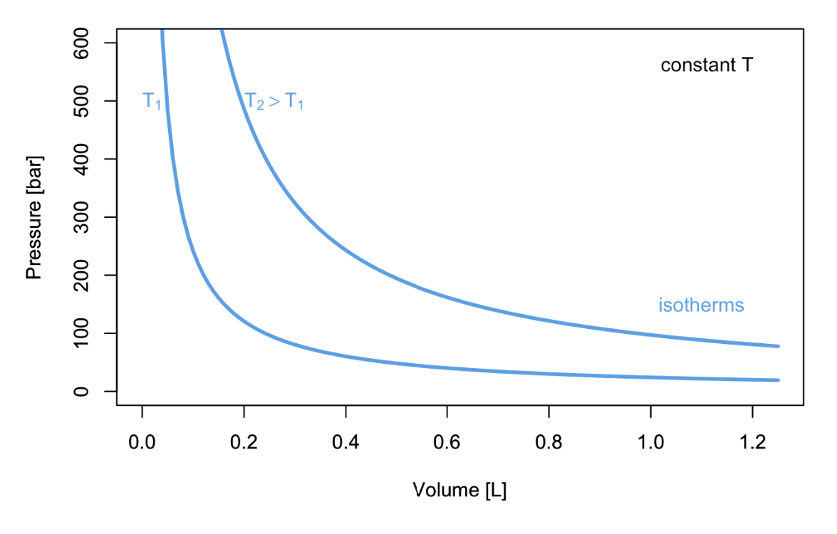
In 1662 Robert Boyle (1627–1691) found that the pressure and the volume of an ideal gas are inversely related at constant temperature. Boyle’s Law has the following mathematical description:
\[ P\propto\dfrac{1}{V}\quad\text{at const.}\;T, \label{11.1.1} \]
or, in other terms:
\[ PV=k_1\quad\text{at const.}\;T, \label{11.1.2} \]
which results in the familiar \(PV\) plots of Figure \(\PageIndex{1}\). As we already discussed in chapter 2, each of the curves in Figure \(\PageIndex{1}\) is obtained at constant temperature, and it is therefore called “isotherm.”
Charles’s and Gay-Lussac’s Laws
It took scientists more than a century to expand Boyle’s work and study the relationship between volume and temperature. In 1787 Jacques Alexandre César Charles (1746–1823) wrote the relationship known as Charles’s Law:
\[ V\propto T\quad\text{at const.}\;P, \label{11.1.3} \]
or, in other terms:
\[ V=k_2 T\quad\text{at const.}\;P, \label{11.1.4} \]
which results in the plots of Figure \(\PageIndex{2}\). Each of the curves is obtained at constant pressure, and it is termed “isobar.”

The interesting thing about isobars is that each line seems to converge to a specific point along the temperature line when we extrapolate them to \(V\rightarrow 0\). This led to the introduction of the absolute temperature scale, suggesting that the temperature will never get smaller than \(-273.15^\circ\mathrm{C}\).
It took an additional 21 years to write a formal relationship between pressure and temperature. The following relationships were proposed by Joseph Louis Gay-Lussac (1778–1850) in 1808:
\[ P\propto T\quad\text{at const.}\;V, \label{11.1.5} \]
or, in other terms:
\[ P=k_3 T\quad\text{at const.}\;V, \label{11.1.6} \]
which results in the plots of Figure \(\PageIndex{3}\). Each of the curves is obtained at constant volume, and it is termed “isochor.”

Avogadro’s Law
Ten years later, Amedeo Avogadro (1776–1856) discovered a seemingly unrelated principle by studying the composition of matter. His Avogadro’s Law encodes the relationship between the number of moles in an ideal gas and its volume as:
\[ V\propto n\quad\text{at const.}\;P,T, \label{11.1.7} \]
or in other terms:
\[ V=k_4 n\quad\text{at const.}\;P,T, \label{11.1.8} \]
The ideal gas Law
Despite all of the ingredients being available for more than 20 years, it’s only in 1834 that Benoît Paul Émile Clapeyron (1799–1864) was finally able to combine them into what is now known as the ideal gas Law. Using the same formulas obtained above, we can write:
\[ PV=\underbrace{k_3 T}_{\text{from Gay-Lussac's}} \cdot \underbrace{k_4 n,}_{\text{from Avogadro's}} \label{11.1.9} \]
which by renaming the product of the two constants \(k_3\) and \(k_4\) as \(R\), becomes:
\[ PV=nRT \label{11.1.10} \]
The value of the constant \(R\) can be determined experimentally by measuring the volume that 1 mol of an ideal gas occupies at a constant temperature (e.g., at \(T=0^\circ\mathrm{C}\)) and a constant pressure (e.g., atmospheric pressure \(P=1\;\mathrm{atm}\)). At those conditions, the volume is measured at 22.4 L, resulting in the following value of \(R\):
\[ R=\dfrac{VP}{nT}=\dfrac{22.4 \cdot 1}{1 \cdot 273}=0.082 \;\dfrac{\text{L atm}}{\text{mol K}}, \label{11.1.11} \]
which a simple conversion to SI units transforms into:
\[ R=8.31\;\dfrac{\text{J}}{\text{mol K}}. \label{11.1.12} \]