8.78: A Simple Quantum Computer

Giving a friend directions to his house, Yogi Berra said “When you come to a fork in the road, take it.” I will attempt to demonstrate that this well-known “yogi-ism” describes an essential feature of quantum phenomena and the parallelism that is exploited by a quantum computer.

A Mach-Zehnder interferometer (MZI) is a simple example of a quantum computer. Its main components are two optical beam splitters (think half-silvered mirrors). The first, the fork in the road, creates a superposition of two computational paths. The second beam splitter recombines the paths giving rise to the constructive and destructive interference that is essential to quantum computation.

The MZI quantum computer will be assembled in three steps. The first step shows a 50-50 beam splitter that can be illuminated by two input ports and their vector designations, |0> and |1>. Since we are dealing with computation it will eventually be shown that a 50-50 beam splitter is a square root of NOT gate - √NOT. The quantum aspects of computation are already appearing because there is no classical analog for a √NOT gate, and yet it exists physically as a simple 50-50 beam splitter.

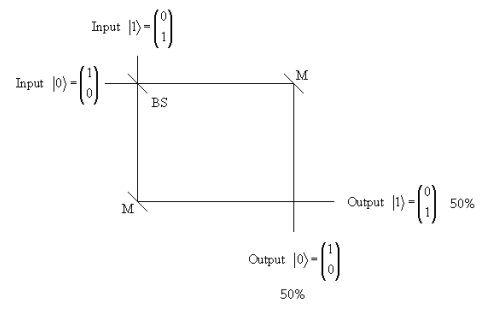
The experimental results for illuminating ports |0> and |1> are reported in the table below. From a classical respective there is nothing unusual here. A 50-50 beam splitter transmits 50% of the radiation and reflects 50% of the radiation illuminating it. Even if we adopt the photon concept and consider many single photon events, there is still nothing worthy of comment. Statistically half the photons are transmitted and half reflected, no matter which input port is used. And the results are totally random. We cannot predict with certainty the results of individual events. We only know that if we record a statistically meaningful number of results this is what we get.

\[ \begin{array}{|c|c|c|c|c|} \hline \\ |0 \rangle \text{ Input} & |0 \rangle & \text{Transmitted} & |0 \rangle & 50 \% \\ \hline \\ |0 \rangle \text{ Input} & |0 \rangle & \text{Reflected} & |1 \rangle & 50 \% \\ \hline \\ |1 \rangle \text{ Input} & |1 \rangle & \text{Reflected} & |0 \rangle & 50 \% \\ \hline \\ |1 \rangle \text{ Input} & |1 \rangle & \text{Transmitted} & |1 \rangle & 50 \% \\ \hline \end{array} \nonumber \]

At this point we could interpret these results as saying that the source emits photons and the detector registers photons, and that the events at the beam splitter are random; we cannot predict with certainty the outcome of any single encounter of a photon with the beam splitter, only the statistical results given in the table.

Quantum mechanically, the beam splitter is Yogi’s fork in the road, and the photon as a quantum mechanical object (quon) takes both paths. The photon paths, |0> and |1>, are represented by the vectors in the figure. The beam splitter’s interaction with a photon is given by the following matrix. By convention the probability amplitude for transmission is 1/√2 and for reflection it is i/√2. In other words, a 90 degree phase change is assigned to reflection at the beam splitter.

\[ \widehat{BS} = \widehat{ \sqrt{NOT}} = \frac{1}{ \sqrt{2}} \begin{pmatrix} 1 & i \\ i & 1 \end{pmatrix} \nonumber \]

Thus, according to simple matrix algebra the consequence of a photon’s interaction with a 50-50 beam splitter is the creation of a quantum mechanical superposition of the photon being present simultaneously in both paths.

\[ \begin{matrix} \widehat{BS} |0 \rangle = \frac{1}{ \sqrt{2}} \begin{pmatrix} 1 & i \\ i & 1 \end{pmatrix} \begin{pmatrix} 1 \\ 0 \end{pmatrix} = \frac{1}{ \sqrt{2}} \begin{pmatrix} 1 \\ i \end{pmatrix} = \frac{1}{ \sqrt{2}} \left[ \begin{pmatrix} 1 \\ 0 \end{pmatrix} + i \begin{pmatrix} 0 \\ 1 \end{pmatrix} \right] = \frac{1}{ \sqrt{2}} \left[ |0 \rangle + i |1 \rangle \right] \\ \widehat{BS} |1 \rangle = \frac{1}{ \sqrt{2}} \begin{pmatrix} 1 & i \\ i & 1 \end{pmatrix} \begin{pmatrix} 0 \\ 1 \end{pmatrix} = \frac{1}{ \sqrt{2}} \begin{pmatrix} i \\ 1 \end{pmatrix} = \frac{1}{ \sqrt{2}} \left[ i \begin{pmatrix} 1 \\ 0 \end{pmatrix} + \begin{pmatrix} 0 \\ 1 \end{pmatrix} \right] = \frac{1}{ \sqrt{2}} \left[ |0 \rangle + i |1 \rangle \right] \end{matrix} \nonumber \]

According to quantum mechanics, the photon is in an even superposition of being transmitted and reflected after the beam splitter. The probability of being detected in either output channel is the absolute square of the probability amplitudes, as calculated below.

\[ \left| \frac{1}{ \sqrt{2}} \right|^2 = \left| \frac{i}{ \sqrt{2}} \right|^2 = \frac{1}{2} \nonumber \]

From the quantum mechanical perspective, we say that upon observation or detection the superposition collapses into one of its classical possibilities. This interpretation of a simple experiment might seem a bit extravagant, until we proceed to the next step which involves the insertion of a second beam splitter at the intersection of the two output channels.

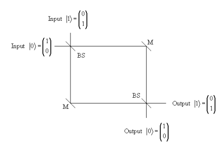
Now there are two paths to each output channel. The first beam splitter creates two paths, one to each detector (output channel), the second beam splitter recombines those paths giving two ways to reach each detector. This is a simple example of Feynman’s “sum over histories” approach to quantum mechanics. We now have the possibility that the probability amplitudes for these “histories” or paths will interfere constructively or destructively, and of course they do.

\[ \begin{array}{|c|c|c|c|} \hline \\ \text{Input} & \text{History} & \text{Output} & \text{Probability} \\ \hline \\ |0 \rangle & \text{TT + RR} & |0 \rangle & 0 \% \\ \hline \\ |1 \rangle & \text{TR + RT} & |0 \rangle & 100 \% \\ \hline \\ |1 \rangle & \text{TT + RR} & |1 \rangle & 0 \% \\ \hline \end{array} \nonumber \]

Note the strikingly different results from that with a single beam splitter. Now |0> input never yields |0> output, and |1> input never yields |1> output. That’s why a beam splitter is called a √NOT gate - √NOT√NOT = NOT.

\[ \widehat{NOT} = \widehat{ \sqrt{NOT}} \widehat{ \sqrt{NOT}} = \frac{1}{ \sqrt{2}} \begin{pmatrix} 1 & i \\ i & 1 \end{pmatrix} \frac{1}{ \sqrt{2}} \begin{pmatrix} 1 & i \\ i & 1 \end{pmatrix} = i \begin{pmatrix} 0 & 1 \\ 1 & 0 \end{pmatrix} \nonumber \]

The operation of the NOT gate on the two possible input states is as follows: the probability that input |0> will yield output |1> is |i|2 = 1, and, of course the probability that input |1> will yield output |0> is the same.

\[ \begin{matrix} \widehat{NOT} |0 \rangle = i \begin{pmatrix} 0 & 1 \\ 1 & 0 \end{pmatrix} \begin{pmatrix} 1 \\ 0 \end{pmatrix} = i \begin{pmatrix} 0 \\ 1 \end{pmatrix} = i |1 \rangle \\ \widehat{NOT} |1 \rangle = i \begin{pmatrix} 0 & 1 \\ 1 & 0 \end{pmatrix} \begin{pmatrix} 0 \\ 1 \end{pmatrix} = i \begin{pmatrix} 1 \\ 0 \end{pmatrix} = i |0 \rangle \end{matrix} \nonumber \]

This is a matrix mechanics calculation. It is also instructive to use Feynman’s “sum over histories” approach explicitly. There we sum the probability amplitudes for each history or path and take the square of the absolute magnitude. Recall that the probability amplitudes are 1/√2 and i/√2 for transmission and reflection, respectively.

\[ \begin{matrix} |0 \rangle \xrightarrow{TT+RR} |0 \rangle \left| \frac{1}{ \sqrt{2}} \frac{1}{ \sqrt{2}} + \frac{i}{ \sqrt{2}} \frac{i}{ \sqrt{2}} \right|^2 = 0 & |0 \rangle \xrightarrow{TR+RT} |1 \rangle \left| \frac{i}{ \sqrt{2}} \frac{1}{ \sqrt{2}} + \frac{i}{ \sqrt{2}} \frac{1}{ \sqrt{2}} \right|^2 = 1 \\ |1 \rangle \xrightarrow{TT+RR} |1 \rangle \left| \frac{1}{ \sqrt{2}} \frac{1}{ \sqrt{2}} + \frac{i}{ \sqrt{2}} \frac{i}{ \sqrt{2}} \right|^2 = 0 & |1 \rangle \xrightarrow{TR+RT} |0 \rangle \left| \frac{1}{ \sqrt{2}} \frac{i}{ \sqrt{2}} + \frac{i}{ \sqrt{2}} \frac{1}{ \sqrt{2}} \right|^2 = 1 \end{matrix} \nonumber \]

For \( |0 \rangle \rightarrow |0 \rangle\) and \( |1 \rangle \rightarrow |1 \rangle\) the probability amplitudes for the paths (histories) interfere destructively, while for \( |0 \rangle \rightarrow |1 \rangle\) and \( |1 \rangle \rightarrow |0 \rangle\) they interfere constructively.

Now we are ready to see how a modified Mach-Zehnder interferometer can function as a quantum computer. But first a simple non-mathematical example will be examined.

Suppose you are asked whether two pieces of glass are the same thickness. Most likely you would use a caliper to measure the individual pieces and then compare the measurements. This is a bit of overkill because you were only asked if pieces of glass are the same thickness, not what the individual thicknesses are.

The question can be answered with a single measurement by placing the pieces of glass in opposite arms of the MZI as shown in the figure.

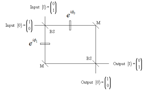
The speed of light in glass differs from that in air. Therefore the pieces of glass will cause phase shifts that depend on their thickness. This is the origin of the exponential terms in the figure. For example,

\[ \phi_0 = 2 \pi \frac{ \delta_0}{ \lambda} \nonumber \]

is the phase shift (in radians) in the |0> arm of the interferometer. Here δ0 is the glass thickness and λ is the wavelength of the light. Recall that in the absence of the glass, the probability for |0> input to |0> output is zero. In the presence of the glass, using Feynman’s sum over histories to calculate the probability yields the following expression.

\[ \left| \frac{1}{ \sqrt{2}} e^{i \phi_0} \frac{1}{ \sqrt{2}} + \frac{i}{ \sqrt{2}} e^{i \phi_1} \frac{i}{ \sqrt{2}} \right|^2 \nonumber \]

We see that only if the phase changes are the same (glass thickness the same) in both arms of the interferometer is the \( |0 \rangle \rightarrow |0 \rangle\) probability zero. If light emerges from the |0> output channel we know that the pieces of glass are not the same thickness, and have answered the thickness question with a single measurement.

This is a precursor to the proof of principle example David Deutsch provided for the quantum computer (see primary reference cited below). In his example, Deutsch proposed a binary function f that maps {0,1} to {0,1} for which there are four possibilities: f(0) = 0, f(0) = 1, f(1) = 0, and f(1) = 1. The question is (analogous to the glass thickness question) are f(0) and f(1) the same or different? Classically two calculations of f are required, one with input 0 and one with input 1. The modified MZI shown below illustrates how the answer can be achieved with a single parallel calculation. In other words, a photon transverses both arms of the interferometer and its output destination answers the question.

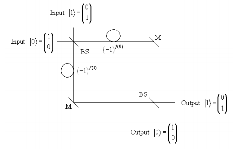
The delay loops replace the pieces of glass and cause a 1800 phase shift if taken (180⁰ = π; exp(iπ) = - 1). Whether they are taken is controlled by the value of f. If its value is 0 the loop is bypassed, if its value is 1 the loop is taken bringing about a 180⁰ phase change in that arm of the interferometer.

Feynman’s method provides the following results. The probability for \( |0 \rangle \rightarrow |0 \rangle\) is 0 if f(0) = f(1) and 1 if f(0) ≠ f(1).

\[ \left| \frac{1}{ \sqrt{2}} (-1)^{f(0)} \frac{1}{ \sqrt{2}} + \frac{i}{ \sqrt{2}} (-1)^{f(1)} \frac{i}{ \sqrt{2}} \right|^2 = \left| \frac{1}{2} \left[ (-1)^{f(0)} - (-1)^{f(1)} \right] \right|^2 = \begin{Bmatrix} 0 = \text{ if} f(0) = f(1) \\ 1 = \text{ if} f(0) \neq f(1) \end{Bmatrix} \nonumber \]

Consequently the probability for \( |0 \rangle \rightarrow |1 \rangle\) is 1 if f(0) = f(1) and 0 if f(0) ≠ f(1).

\[ \left| \frac{1}{ \sqrt{2}} (-1)^{f(0)} \frac{i}{ \sqrt{2}} + \frac{i}{ \sqrt{2}} (-1)^{f(1)} \frac{1}{ \sqrt{2}} \right|^2 = \left| \frac{1}{2} \left[ (-1)^{f(0)} - (-1)^{f(1)} \right] \right|^2 = \begin{Bmatrix} 1 = \text{ if} f(0) = f(1) \\ 0 = \text{ if} f(0) \neq f(1) \end{Bmatrix} \nonumber \]

In summary, a single output measurement answers the initial question. We might think of this as an example of mathematical multitasking. A Mach-Zehnder interferometer creates a superposition of two computational paths providing the opportunity for the constructive and destructive interference that is the essential characteristic of quantum computation.

Primary reference:

Machines, Logic and Quantum Physics

David Deutsch, Artur Ekert, and Rossella Lupacchini

arXiv:math.HO/9911150 v1; 19 November 1999

Other sources:

The Quest for the Quantum Computer

Julian Brown

Simon & Schuster, 2000

Quantum Mechanical Computers

Richard P. Feynman

Foundations of Physics 16, 507-531 (1985)

Quantum Information and Computation

Charles H. Bennett

Physics Today, October 1995, pp 24-30

Quantum Computers

T. D. Ladd, et al.

Nature, 4 March 2010, pp 45-53