
8.43: Another Summary of Fenyman's "Stimulating Physics with Computers"
- Page ID
- 144086

This tutorial is based on "Simulating Physics with Computers" by Richard Feynman, published in the International Journal of Theoretical Physics (volume 21, pages 481-485), and Julian Brown's Quest for the Quantum Computer (pages 91-100). Feynman used the experiment outlined below to establish that a local classical computer could not simulate quantum physics.
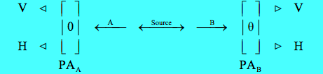
A two-stage atomic cascade emits entangled photons (A and B) in opposite directions with the same circular polarization according to observers in their path.
\[ | \Psi \rangle = \frac{1}{ \sqrt{2}} \left[ |L \rangle_A |L \rangle_B + |R \rangle_A | \rangle_B \right] \nonumber \]
The experiment involves the measurement of photon polarization states in the vertical/horizontal measurement basis, and allows for the rotation of the right-hand detector through an angle θ, in order to explore the consequences of quantum mechanical entanglement. PA stands for polarization analyzer and could simply be a calcite crystal.
As mentioned above the photon polarization measurements are made in the V-H basis. The L and R polarization states are superpositions of the V and H polarization states, enabling the original state to be written in the measurement basis.
\[ \begin{matrix} | L \rangle = \frac{1}{ \sqrt{2}} \left[ | V \rangle + i | H \rangle \right] & | R \rangle = \frac{1}{ \sqrt{2}} \left[ | V \rangle - i | H \rangle \right] & | \Psi \rangle = \frac{1}{ \sqrt{2}} \left[ | V \rangle_A | V \rangle_B - | H \rangle_A |H \rangle_B \right] \end{matrix} \nonumber \]
Rotating the right-hand polarizer counter-clockwise by θ yields the following polarization states for B.
\[ \begin{matrix} | V\ \rangle_B = \cos \theta | V \rangle_B - \sin \theta |H \rangle_B & | H' \rangle_B = \sin \theta | V \rangle_B + \cos \theta | H \rangle_B \end{matrix} \nonumber \]
After rotation of B's analyzer the four measurement outcomes, both photons vertically polarized, both horizontally polarized, one vertical and the other horizontal, are expressed mathematically below.
\[ \begin{matrix} | \Psi_{VV'} \rangle = | V \rangle_A |V' \rangle_B & | \Psi_{VH'} \rangle = |V \rangle_A | H' \rangle_B & | \Psi_{HV'} \rangle = |H \rangle_A | V' \rangle_B & | \Psi_{HH'} \rangle = |H \rangle_A | H' \rangle_B \end{matrix} \nonumber \]
Using the equations provided the probability the photons will behave the same way, both vertically polarized or both horizontally polarized is cos2(θ).
\[ \left| \left\langle \Psi_{VV'} | \Psi \right\rangle \right|^2 + \left| \right|^2 = \cos^2 \theta \nonumber \]
Next the probability the photons will behave the same is calculated for three values of θ.
\[ P_{same} \theta = \cos ( \theta)^2 & P_{same} (0 \text{ deg}) = 1 & P_{same} (90 \text{ deg} = 0 & P_{same} (30 \text{ deg}) = 0.75 \nonumber \]
These quantum calculations are in agreement with experimental results, but cannot be explained by a local realistic hidden-variable model of reality.
If objects have well-defined properties independent of measurement or observation, the first two results (θ = 0 degrees, θ = 90 degrees) require that the photons carry the following instruction sets, where the hexagonal vertices refer to θ values of 0, 30, 60, 90, 120, and 150 degrees. There are eight possible instruction sets, six of the type on the left and two of the type on the right. The white circles represent vertical polarization and the black circles represent horizontal polarization. In any given measurement, according to local realism, both photons (A and B) carry identical instruction sets, in other words the same one of the eight possible sets.
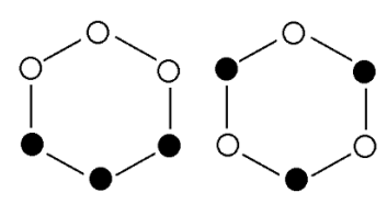
The problem is that while these instruction sets are in agreement with the 0 and 90 degree results, they can't explain the 30 degree data. The figure on the left shows that the same result should be obtained 2/3 of the time (4/6) and the figure on the right never. Thus, local realism predicts that the same result should be obtained 50% of the time, as opposed to the actual result of 75% agreement.
\[ \left( 6 \frac{2}{3} + 2(0) \right) \div 8 = 50 \% \nonumber \]
When Feynman gets to this point in "Simulating Physics with Computers" he writes,
That's all. That's the difficulty. That's why quantum mechanics can't seem to be imitable by a local classical computer.
A local classical computer manipulates bits which are in well-defined states, 0s and 1s, shown above graphically in white and black. However, these classical states are incompatible with the quantum mechanical analysis which is in agreement with experimental results. This two-photon experiment demonstrates that simulation of quantum physics requires a computer that can manipulate 0s and 1s, superpositions of 0 and 1, and entangled superpositions of 0s and 1s. Simulation of quantum physics requires a quantum computer!
Earlier in his paper Feynman sharpened the focus of his analysis by saying "But the physical world is quantum mechanical, and therefore the proper problem is the simulation of quantum physics ..."
He ends his presentation with the following remark.
And I'm not happy with all the analyses that go with just the classical theory, because nature isn't classical, dammit, and if you want to make a simulation of nature, you'd better make it quantum mechanical, ...