
8.4: Another Look at Quantum Teleportation
- Page ID
- 142875

\( \newcommand{\vecs}[1]{\overset { \scriptstyle \rightharpoonup} {\mathbf{#1}} } \)
\( \newcommand{\vecd}[1]{\overset{-\!-\!\rightharpoonup}{\vphantom{a}\smash {#1}}} \)
\( \newcommand{\dsum}{\displaystyle\sum\limits} \)
\( \newcommand{\dint}{\displaystyle\int\limits} \)
\( \newcommand{\dlim}{\displaystyle\lim\limits} \)
\( \newcommand{\id}{\mathrm{id}}\) \( \newcommand{\Span}{\mathrm{span}}\)
( \newcommand{\kernel}{\mathrm{null}\,}\) \( \newcommand{\range}{\mathrm{range}\,}\)
\( \newcommand{\RealPart}{\mathrm{Re}}\) \( \newcommand{\ImaginaryPart}{\mathrm{Im}}\)
\( \newcommand{\Argument}{\mathrm{Arg}}\) \( \newcommand{\norm}[1]{\| #1 \|}\)
\( \newcommand{\inner}[2]{\langle #1, #2 \rangle}\)
\( \newcommand{\Span}{\mathrm{span}}\)
\( \newcommand{\id}{\mathrm{id}}\)
\( \newcommand{\Span}{\mathrm{span}}\)
\( \newcommand{\kernel}{\mathrm{null}\,}\)
\( \newcommand{\range}{\mathrm{range}\,}\)
\( \newcommand{\RealPart}{\mathrm{Re}}\)
\( \newcommand{\ImaginaryPart}{\mathrm{Im}}\)
\( \newcommand{\Argument}{\mathrm{Arg}}\)
\( \newcommand{\norm}[1]{\| #1 \|}\)
\( \newcommand{\inner}[2]{\langle #1, #2 \rangle}\)
\( \newcommand{\Span}{\mathrm{span}}\) \( \newcommand{\AA}{\unicode[.8,0]{x212B}}\)
\( \newcommand{\vectorA}[1]{\vec{#1}} % arrow\)
\( \newcommand{\vectorAt}[1]{\vec{\text{#1}}} % arrow\)
\( \newcommand{\vectorB}[1]{\overset { \scriptstyle \rightharpoonup} {\mathbf{#1}} } \)
\( \newcommand{\vectorC}[1]{\textbf{#1}} \)
\( \newcommand{\vectorD}[1]{\overrightarrow{#1}} \)
\( \newcommand{\vectorDt}[1]{\overrightarrow{\text{#1}}} \)
\( \newcommand{\vectE}[1]{\overset{-\!-\!\rightharpoonup}{\vphantom{a}\smash{\mathbf {#1}}}} \)
\( \newcommand{\vecs}[1]{\overset { \scriptstyle \rightharpoonup} {\mathbf{#1}} } \)
\(\newcommand{\longvect}{\overrightarrow}\)
\( \newcommand{\vecd}[1]{\overset{-\!-\!\rightharpoonup}{\vphantom{a}\smash {#1}}} \)
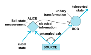
\(\newcommand{\avec}{\mathbf a}\) \(\newcommand{\bvec}{\mathbf b}\) \(\newcommand{\cvec}{\mathbf c}\) \(\newcommand{\dvec}{\mathbf d}\) \(\newcommand{\dtil}{\widetilde{\mathbf d}}\) \(\newcommand{\evec}{\mathbf e}\) \(\newcommand{\fvec}{\mathbf f}\) \(\newcommand{\nvec}{\mathbf n}\) \(\newcommand{\pvec}{\mathbf p}\) \(\newcommand{\qvec}{\mathbf q}\) \(\newcommand{\svec}{\mathbf s}\) \(\newcommand{\tvec}{\mathbf t}\) \(\newcommand{\uvec}{\mathbf u}\) \(\newcommand{\vvec}{\mathbf v}\) \(\newcommand{\wvec}{\mathbf w}\) \(\newcommand{\xvec}{\mathbf x}\) \(\newcommand{\yvec}{\mathbf y}\) \(\newcommand{\zvec}{\mathbf z}\) \(\newcommand{\rvec}{\mathbf r}\) \(\newcommand{\mvec}{\mathbf m}\) \(\newcommand{\zerovec}{\mathbf 0}\) \(\newcommand{\onevec}{\mathbf 1}\) \(\newcommand{\real}{\mathbb R}\) \(\newcommand{\twovec}[2]{\left[\begin{array}{r}#1 \\ #2 \end{array}\right]}\) \(\newcommand{\ctwovec}[2]{\left[\begin{array}{c}#1 \\ #2 \end{array}\right]}\) \(\newcommand{\threevec}[3]{\left[\begin{array}{r}#1 \\ #2 \\ #3 \end{array}\right]}\) \(\newcommand{\cthreevec}[3]{\left[\begin{array}{c}#1 \\ #2 \\ #3 \end{array}\right]}\) \(\newcommand{\fourvec}[4]{\left[\begin{array}{r}#1 \\ #2 \\ #3 \\ #4 \end{array}\right]}\) \(\newcommand{\cfourvec}[4]{\left[\begin{array}{c}#1 \\ #2 \\ #3 \\ #4 \end{array}\right]}\) \(\newcommand{\fivevec}[5]{\left[\begin{array}{r}#1 \\ #2 \\ #3 \\ #4 \\ #5 \\ \end{array}\right]}\) \(\newcommand{\cfivevec}[5]{\left[\begin{array}{c}#1 \\ #2 \\ #3 \\ #4 \\ #5 \\ \end{array}\right]}\) \(\newcommand{\mattwo}[4]{\left[\begin{array}{rr}#1 \amp #2 \\ #3 \amp #4 \\ \end{array}\right]}\) \(\newcommand{\laspan}[1]{\text{Span}\{#1\}}\) \(\newcommand{\bcal}{\cal B}\) \(\newcommand{\ccal}{\cal C}\) \(\newcommand{\scal}{\cal S}\) \(\newcommand{\wcal}{\cal W}\) \(\newcommand{\ecal}{\cal E}\) \(\newcommand{\coords}[2]{\left\{#1\right\}_{#2}}\) \(\newcommand{\gray}[1]{\color{gray}{#1}}\) \(\newcommand{\lgray}[1]{\color{lightgray}{#1}}\) \(\newcommand{\rank}{\operatorname{rank}}\) \(\newcommand{\row}{\text{Row}}\) \(\newcommand{\col}{\text{Col}}\) \(\renewcommand{\row}{\text{Row}}\) \(\newcommand{\nul}{\text{Nul}}\) \(\newcommand{\var}{\text{Var}}\) \(\newcommand{\corr}{\text{corr}}\) \(\newcommand{\len}[1]{\left|#1\right|}\) \(\newcommand{\bbar}{\overline{\bvec}}\) \(\newcommand{\bhat}{\widehat{\bvec}}\) \(\newcommand{\bperp}{\bvec^\perp}\) \(\newcommand{\xhat}{\widehat{\xvec}}\) \(\newcommand{\vhat}{\widehat{\vvec}}\) \(\newcommand{\uhat}{\widehat{\uvec}}\) \(\newcommand{\what}{\widehat{\wvec}}\) \(\newcommand{\Sighat}{\widehat{\Sigma}}\) \(\newcommand{\lt}{<}\) \(\newcommand{\gt}{>}\) \(\newcommand{\amp}{&}\) \(\definecolor{fillinmathshade}{gray}{0.9}\)The purpose of this tutorial is to provide a brief outline of the basic elements of quantum teleportation, as illustrated in the figure below, using matrix and tensor algebra in the Mathcad programming environment. The methods used here are closely related to those presented in the preceding tutorial on teleportation.
As is generally the case, the analysis requires the use of the maximally entangled two‐quibit Bell states, the identity matrix and two of the unitary Pauli matrices.
Bell states:
\[ \Phi_p = \frac{1}{ \sqrt{2}} \begin{pmatrix} 1 \\ 0 \\ 0 \\ 1 \end{pmatrix} \nonumber \]
\[ \Phi_m = \frac{1}{ \sqrt{2}} \begin{pmatrix} 1 \\ 0 \\ 0 \\ -1 \end{pmatrix} \nonumber \]
\[ \Psi_p = \frac{1}{ \sqrt{2}} \begin{pmatrix} 0 \\ 1 \\ 1 \\ 0 \end{pmatrix} \nonumber \]
\[ \Psi_m = \frac{1}{ \sqrt{2}} \begin{pmatrix} 0 \\ 1 \\ -1 \\ 0 \end{pmatrix} \nonumber \]
Identity and x- and z-Pauli matrices:
\[ I = \begin{pmatrix} 1 & 0 \\ 0 & 1 \end{pmatrix} \nonumber \]
\[ \sigma_x = \begin{pmatrix} 0 & 1 \\ 1 & 0 \end{pmatrix} \nonumber \]
\[ \sigma_z = \begin{pmatrix} 1 & 0 \\ 0 & -1 \end{pmatrix} \nonumber \]
Alice wishes to teleport this state to Bob.
\[ \begin{pmatrix} \sqrt{ \frac{1}{3}} \\ \sqrt{ \frac{2}{3}} \end{pmatrix} = \begin{pmatrix} 0.577 \\ 0.816 \end{pmatrix} \nonumber \]
\[ \left[ \left| \begin{pmatrix} \sqrt{ \frac{1}{3}} \\ \sqrt{ \frac{2}{3}} \end{pmatrix} \right| \right]^2 = 1 \nonumber \]
They prepare the first Bell state (Φp) in which Alice has the first qubit and Bob the second. Alice arranges for the state to be teleported and her entangled qubit to meet creating the following three qubit state.
\[ \begin{pmatrix} 0.577 \\ 0.816 \end{pmatrix} \frac{1}{ \sqrt{2}} \begin{pmatrix} 1 \\ 0 \\ 0 \\ 1 \end{pmatrix} \nonumber \]
\[ \Psi = \frac{1}{ \sqrt{2}} \begin{pmatrix} 0.577 \\ 0 \\ 0 \\ 0.577 \\ 0.816 \\ 0 \\ 0 \\ 0.816 \end{pmatrix} \nonumber \]
\[ \Psi^T \Psi = 1 \nonumber \]
Next Alice performs a Bell‐state measurement, in other words she projects Ψ onto the Bell‐state basis given above. The four equally likely outcomes are calculated below. But first letʹs use Φp as an example. Its projector is |Φp >< Φp|.
\[ \Phi _p \Phi _p ^T = \begin{pmatrix} 0.5 & 0 & 0 & 0.5 \\ 0 & 0 & 0 & 0 \\ 0 & 0 & 0 & 0 \\ 0.5 & 0 & 0 & 0.5 \end{pmatrix} \nonumber \]
However, Ψ is a three‐qubit state in which Alice has the first two qubits and Bob the third. In other words, the projector does not operate directly on Bobʹs qubit. Thus the appropriate matrix for this operation uses the identity matrix to leave Bobʹs qubit alone. Kronecker is Mathcadʹs command for tensor multiplication of matrices.
\[ \text{kronecker} ( \Phi_p, \Phi_p,^T, I) = \begin{pmatrix} 0.5 & 0 & 0 & 0 & 0 & 0 & 0.5 & 0 \\ 0 & 0.5 & 0 & 0 & 0 & 0 & 0 & 0.5 \\ 0 & 0 & 0 & 0 & 0 & 0 & 0 & 0 \\ 0 & 0 & 0 & 0 & 0 & 0 & 0 & 0 \\ 0 & 0 & 0 & 0 & 0 & 0 & 0 & 0 \\ 0 & 0 & 0 & 0 & 0 & 0 & 0 & 0 \\ 0.5 & 0 & 0 & 0 & 0 & 0 & 0.5 & 0 \\ 0 & 0.5 & 0 & 0 & 0 & 0 & 0 & 0.5 \end{pmatrix} \nonumber \]
Next we show that indeed there are four equally likely outcomes for the Bell-state measurement.
\[ \left( \left| \text{kronecker} \left( \Phi_p, \Phi_p^T, I \right) \Psi \right| \right)^2 = 0.25 \nonumber \]
\[ \left( \left| \text{kronecker} \left( \Phi_m, \Phi_m^T, I \right) \Psi \right| \right)^2 = 0.25 \nonumber \]
\[ \left( \left| \text{kronecker} \left( \Psi_p, \Psi_p^T, I \right) \Psi \right| \right)^2 = 0.25 \nonumber \]
\[ \left( \left| \text{kronecker} \left( \Psi_m, \Psi_m^T, I \right) \Psi \right| \right)^2 = 0.25 \nonumber \]
Aliceʹs Bell‐state measurement yields one of these results, which she communicates to Bob through a classical channel. As shown below, depending on Aliceʹs report Bob carries out the following unitary operations on his qubit to receive the teleported state: I, σz, σx, and σzσx. The multiplicative factor of 2 normalizes the result of the Bell state measurement.
\[ 2 \text{kronecker} ( \Phi_p, \Phi_p^T, I) \Psi = \begin{pmatrix} 0.408 \\ 0.577 \\ 0 \\ 0 \\ 0 \\ 0 \\ 0.408 \\ 0.577 \end{pmatrix} \nonumber \]
Factors to:
\[ \frac{1}{ \sqrt{2}} \begin{pmatrix} 1 \\ 0 \\ 0 \\ 1 \end{pmatrix} \begin{pmatrix} 0.577 \\ 0.816 \end{pmatrix} \nonumber \]
So Bob does nothing:
\[ I \begin{pmatrix} 0.577 \\ 0.816 \end{pmatrix} = \begin{pmatrix} 0.577 \\ 0.816 \end{pmatrix} \nonumber \]
\[ 2 \text{kronecker} ( \Phi_m, \Phi_m^T, I) \Psi = \begin{pmatrix} 0.408 \\ -0.577 \\ 0 \\ 0 \\ 0 \\ 0 \\ -0.408 \\ 0.577 \end{pmatrix} \nonumber \]
Factors to:
\[ \frac{1}{ \sqrt{2}} \begin{pmatrix} 1 \\ 0 \\ 0 \\ -1 \end{pmatrix} \begin{pmatrix} 0.577 \\ -0.816 \end{pmatrix} \nonumber \]
So Bob does this:
\[ \sigma_z \begin{pmatrix} 0.577 \\ -0.816 \end{pmatrix} = \begin{pmatrix} 0.577 \\ 0.816 \end{pmatrix} \nonumber \]
\[ 2 \text{kronecker} ( \Psi_p, \Psi_p^T, I) \Psi = \begin{pmatrix} 0 \\ 0 \\ 0.577 \\ 0.408 \\ 0.577 \\ 0.408 \\ 0 \\ 0 \end{pmatrix} \nonumber \]
Factors to:
\[ \frac{1}{ \sqrt{2}} \begin{pmatrix} 0 \\ 1 \\ 1 \\ 0 \end{pmatrix} \begin{pmatrix} 0.816 \\ 0.577 \end{pmatrix} \nonumber \]
So Bob does this:
\[ \sigma_x \begin{pmatrix} 0.816 \\ 0.577 \end{pmatrix} = \begin{pmatrix} 0.577 \\ 0.816 \end{pmatrix} \nonumber \]
\[ 2 \text{kronecker} ( \Psi_m, \Psi_m^T, I) \Psi = \begin{pmatrix} 0 \\ 0 \\ -0.577 \\ 0.408 \\ 0.577 \\ 0.408 \\ 0 \\ 0 \end{pmatrix} \nonumber \]
Factors to:
\[ \frac{1}{ \sqrt{2}} \begin{pmatrix} 0 \\ 1 \\ 1 \\ 0 \end{pmatrix} \begin{pmatrix} 0.816 \\ 0.577 \end{pmatrix} \nonumber \]
So Bob does this:
\[ \sigma_x \begin{pmatrix} 0.816 \\ 0.577 \end{pmatrix} = \begin{pmatrix} 0.577 \\ 0.816 \end{pmatrix} \nonumber \]
Of course, only 25% of the time is the state of Aliceʹs photon teleported to Bob without further action on his part. Note that we began with Alice and Bob sharing the p Bell state. Consequently when Aliceʹs Bell state measurement yields Φp, Bob has Aliceʹs photon. We now show that teleportation can be presented quite simply using the density matrix formulation under this circumstance.
Bell state measurement result (normalized):
\[ 2 \text{kronecker} ( \Phi_p, \Phi_p^T, I) \Psi = \begin{pmatrix} 0.408 \\ 0.577 \\ 0 \\ 0 \\ 0 \\ 0 \\ 0.408 \\ 0.577 \end{pmatrix} \nonumber \]
Density matrix of measurement state:
\[ \begin{pmatrix} 0.408 \\ 0.577 \\ 0 \\ 0 \\ 0 \\ 0 \\ 0.408 \\ 0.577 \end{pmatrix} \begin{pmatrix} 0.408 \\ 0.577 \\ 0 \\ 0 \\ 0 \\ 0 \\ 0.408 \\ 0.577 \end{pmatrix}^T = \begin{pmatrix} 0.166 & 0.235 & 0 & 0 & 0 & 0 & 0.166 & 0.235 \\ 0.235 & 0.333 & 0 & 0 & 0 & 0 & 0.235 & 0.333 \\ 0 & 0 & 0 & 0 & 0 & 0 & 0 & 0 \\ 0 & 0 & 0 & 0 & 0 & 0 & 0 & 0 \\ 0 & 0 & 0 & 0 & 0 & 0 & 0 & 0 \\ 0 & 0 & 0 & 0 & 0 & 0 & 0 & 0 \\ 0.166 & 0.235 & 0 & 0 & 0 & 0 & 0.166 & 0.235 \\ 0.235 & 0.333 & 0 & 0 & 0 & 0 & 0.235 & 0.333 \end{pmatrix} \nonumber \]
Next the density matrix is calculated assuming Bob has the teleported state. The density matrices are identical confirming that Aliceʹs initial state has been successfully teleported to Bob.
\[ \text{kronecker} \left[ \Phi_p, \Phi_p^T, \begin{pmatrix} 0.577 \\ 0.816 \end{pmatrix} \begin{pmatrix} 0.577 \\ 0.816 \end{pmatrix} ^T \right] \begin{pmatrix} 0.166 & 0.235 & 0 & 0 & 0 & 0 & 0.166 & 0.235 \\ 0.235 & 0.333 & 0 & 0 & 0 & 0 & 0.235 & 0.333 \\ 0 & 0 & 0 & 0 & 0 & 0 & 0 & 0 \\ 0 & 0 & 0 & 0 & 0 & 0 & 0 & 0 \\ 0 & 0 & 0 & 0 & 0 & 0 & 0 & 0 \\ 0 & 0 & 0 & 0 & 0 & 0 & 0 & 0 \\ 0.166 & 0.235 & 0 & 0 & 0 & 0 & 0.166 & 0.235 \\ 0.235 & 0.333 & 0 & 0 & 0 & 0 & 0.235 & 0.333 \end{pmatrix} \nonumber \]