5.20: Electron Diffraction at Multiple Slits
- Page ID
- 150545

\( \newcommand{\vecs}[1]{\overset { \scriptstyle \rightharpoonup} {\mathbf{#1}} } \)
\( \newcommand{\vecd}[1]{\overset{-\!-\!\rightharpoonup}{\vphantom{a}\smash {#1}}} \)
\( \newcommand{\id}{\mathrm{id}}\) \( \newcommand{\Span}{\mathrm{span}}\)
( \newcommand{\kernel}{\mathrm{null}\,}\) \( \newcommand{\range}{\mathrm{range}\,}\)
\( \newcommand{\RealPart}{\mathrm{Re}}\) \( \newcommand{\ImaginaryPart}{\mathrm{Im}}\)
\( \newcommand{\Argument}{\mathrm{Arg}}\) \( \newcommand{\norm}[1]{\| #1 \|}\)
\( \newcommand{\inner}[2]{\langle #1, #2 \rangle}\)
\( \newcommand{\Span}{\mathrm{span}}\)
\( \newcommand{\id}{\mathrm{id}}\)
\( \newcommand{\Span}{\mathrm{span}}\)
\( \newcommand{\kernel}{\mathrm{null}\,}\)
\( \newcommand{\range}{\mathrm{range}\,}\)
\( \newcommand{\RealPart}{\mathrm{Re}}\)
\( \newcommand{\ImaginaryPart}{\mathrm{Im}}\)
\( \newcommand{\Argument}{\mathrm{Arg}}\)
\( \newcommand{\norm}[1]{\| #1 \|}\)
\( \newcommand{\inner}[2]{\langle #1, #2 \rangle}\)
\( \newcommand{\Span}{\mathrm{span}}\) \( \newcommand{\AA}{\unicode[.8,0]{x212B}}\)
\( \newcommand{\vectorA}[1]{\vec{#1}} % arrow\)
\( \newcommand{\vectorAt}[1]{\vec{\text{#1}}} % arrow\)
\( \newcommand{\vectorB}[1]{\overset { \scriptstyle \rightharpoonup} {\mathbf{#1}} } \)
\( \newcommand{\vectorC}[1]{\textbf{#1}} \)
\( \newcommand{\vectorD}[1]{\overrightarrow{#1}} \)
\( \newcommand{\vectorDt}[1]{\overrightarrow{\text{#1}}} \)
\( \newcommand{\vectE}[1]{\overset{-\!-\!\rightharpoonup}{\vphantom{a}\smash{\mathbf {#1}}}} \)
\( \newcommand{\vecs}[1]{\overset { \scriptstyle \rightharpoonup} {\mathbf{#1}} } \)
\( \newcommand{\vecd}[1]{\overset{-\!-\!\rightharpoonup}{\vphantom{a}\smash {#1}}} \)
The American Journal of Physics published a translation of Claus Jonsson's paper "Electron Diffraction at Multiple Slits" in American Journal of Physics 42, 4-11 (1974). The following calculations are in agreement with the diffraction patterns reported by Jonsson.
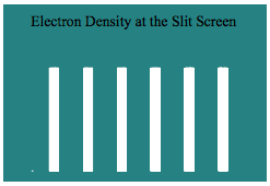
\[ \begin{matrix} \text{Number of slits:} & n = 6 & \text{Slit width:} & w = .5 \\ \text{Slit locations:} & s_1 = 0 & s_2 = 2 & s_3 = 4 & s_4 = 6 & s_5 = 8 & s_6 = 10 \end{matrix} \nonumber \]
Normalized coordinate-space wave function at the slit screen:
\[ \Psi (x) = \frac{1}{ \sqrt{N}} \left| \begin{matrix} \frac{1}{ \sqrt{w}} \text{ if } \sum_{j = 1}^{n} \left[ ( x \geq - s_j ) ( x \leq s_j + w ) \right] \\ 0 \text{otherwise} \end{matrix} \right. \nonumber \]
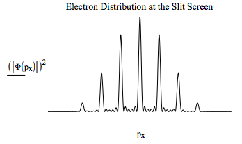
Fourier transform the position wave function into the momentum representation:
\[ \Phi (p_x) = \frac{1}{ \sqrt{2 \pi}} \int_0 ^{s_n + w} exp(-i p_x x) \Psi (x) dx \nonumber \]