3.15: Localized and Delocalized Molecular Orbitals

The generation of localized molecular orbitals (LMOs) from canonical or delocalized molecular orbitals (DMOs) will be illustrated by modeling the π-electrons of 1,3-butadiene as particles in a one-dimensional box (PIB). Solving Schrödinger's equation for this application yields the familiar sine function for the canonical orbitals. The n = 1 and n = 2 states are occupied by two π-electrons each; Ψ and Ψ2 for both states are graphed below.

\[ \begin{matrix} \Psi (n,~x) = \sqrt{2} \sin (n \pi x) & x = 0, .01 .. 1 \end{matrix} \nonumber \]

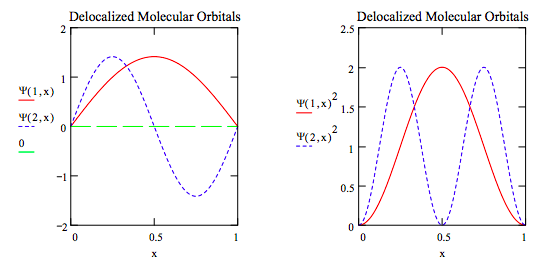
These canonical, delocalized wave functions present a problem for chemists who are accoustomed to localizing the π-electrons of butadiene between carbons 1 and 2, and carbons 3 and 4 with the Lewis structure shown below. In contradiction to this view, the DMOs clearly distribute the π-electron density over the entire carbon backbone

H₂C=CH-CH=CH₂

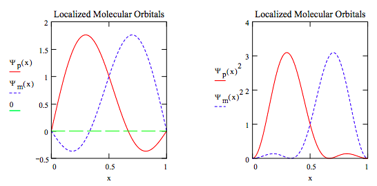
The chemist's localized-electron-pair model can be recovered to some extent from the delocalized, canonical wave functions by invoking the quantum mechanical superposition principle. The superposition principle teaches that any linear combination of the canonical solutions is also a valid wave function as long as they are only used to interpret physical properties that depend on the total electron density. The canonical DMOs are required for single-electron phenomena such as electronic spectroscopy and ionization phenomena.

Thus, it is easy to show that simply adding (Ψ_p) and subtracting (Ψ_m) the canonical wave functions yields LMOs in this simple example involving a particle-in-a-box model for the π-electrons of butadiene. Ψp shifts electron density to the left closer to the bond region between carbon atoms 1 and 2, while Ψ_m shows the electron density closer to the bond region between carbon atoms 3 and 4. Naturally, for more complicated molecular situations a more sophisticated protocol is required to generate LMOs.

\[ \begin{matrix} \Psi_p (x) = \frac{1}{ \sqrt{2}} ( \Psi (1,~x) + \Psi (2,~x)) & \Psi_m (x) = \frac{1}{ \sqrt{2}} ( \Psi (1,~x) - \Psi (2,~x)) \end{matrix} \nonumber \]

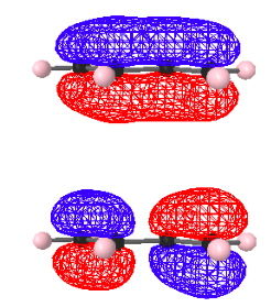
For example, raising the level of theory from PIB to a low-level ab initio quantum mechanical basis set (STO-3G) yields the following HOMO-1 and HOMO for butadiene. These, of course, are the two occupied π molecular orbitals that are equivalent to the n = 1 and n =2 states for the PIB model. Just as for the PIB model the HOMO-1 has no nodes, while the HOMO has one node.

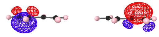
As noted above there are a variety of protocols in use to provide LMOs from the canonical DMOs. A method in wide-spread use forms LMOs from linear combinations of the DMOs by maximizing intra-orbital electron repulsion. This protocol yields the following LMOs for the π electrons in butadiene.

For a more detailed discussion of this subject and useful references to the pedagogical and primary literature consult the following reference. R. Bruce Martin, "Localized and Spectroscopic Orbitals: Squirrel Ears on Water," Journal of Chemical Education, 65(8), 668-670 (1988).