10.38: Variation Method Using the Wigner Function- Finite Potential Well
- Page ID
- 137003

\( \newcommand{\vecs}[1]{\overset { \scriptstyle \rightharpoonup} {\mathbf{#1}} } \)
\( \newcommand{\vecd}[1]{\overset{-\!-\!\rightharpoonup}{\vphantom{a}\smash {#1}}} \)
\( \newcommand{\id}{\mathrm{id}}\) \( \newcommand{\Span}{\mathrm{span}}\)
( \newcommand{\kernel}{\mathrm{null}\,}\) \( \newcommand{\range}{\mathrm{range}\,}\)
\( \newcommand{\RealPart}{\mathrm{Re}}\) \( \newcommand{\ImaginaryPart}{\mathrm{Im}}\)
\( \newcommand{\Argument}{\mathrm{Arg}}\) \( \newcommand{\norm}[1]{\| #1 \|}\)
\( \newcommand{\inner}[2]{\langle #1, #2 \rangle}\)
\( \newcommand{\Span}{\mathrm{span}}\)
\( \newcommand{\id}{\mathrm{id}}\)
\( \newcommand{\Span}{\mathrm{span}}\)
\( \newcommand{\kernel}{\mathrm{null}\,}\)
\( \newcommand{\range}{\mathrm{range}\,}\)
\( \newcommand{\RealPart}{\mathrm{Re}}\)
\( \newcommand{\ImaginaryPart}{\mathrm{Im}}\)
\( \newcommand{\Argument}{\mathrm{Arg}}\)
\( \newcommand{\norm}[1]{\| #1 \|}\)
\( \newcommand{\inner}[2]{\langle #1, #2 \rangle}\)
\( \newcommand{\Span}{\mathrm{span}}\) \( \newcommand{\AA}{\unicode[.8,0]{x212B}}\)
\( \newcommand{\vectorA}[1]{\vec{#1}} % arrow\)
\( \newcommand{\vectorAt}[1]{\vec{\text{#1}}} % arrow\)
\( \newcommand{\vectorB}[1]{\overset { \scriptstyle \rightharpoonup} {\mathbf{#1}} } \)
\( \newcommand{\vectorC}[1]{\textbf{#1}} \)
\( \newcommand{\vectorD}[1]{\overrightarrow{#1}} \)
\( \newcommand{\vectorDt}[1]{\overrightarrow{\text{#1}}} \)
\( \newcommand{\vectE}[1]{\overset{-\!-\!\rightharpoonup}{\vphantom{a}\smash{\mathbf {#1}}}} \)
\( \newcommand{\vecs}[1]{\overset { \scriptstyle \rightharpoonup} {\mathbf{#1}} } \)
\( \newcommand{\vecd}[1]{\overset{-\!-\!\rightharpoonup}{\vphantom{a}\smash {#1}}} \)
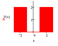
Define potential energy:
\[ V(x) = if[( x \geq -1)(x \leq1), 0, 20 \nonumber \]
Display potential energy:
Choose trial wave function:
\[ \psi (x, \beta ) = \left( \frac{2 \beta}{ \pi} \right)^2 exp( - \beta x^2) \nonumber \]
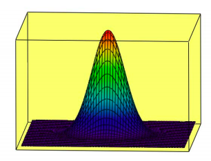
Calculate the Wigner distribution function:
\[ W(x, p, \beta ) = \frac{1}{2 \pi} \int_{- \infty}^{ \infty} \psi \left( x+ \frac{s}{2} , \beta \right) ds \big|_{assume,~ \beta > 0}^{simplify} \rightarrow \frac{1}{ \pi} e^{ \frac{-1}{2} \frac{ 4 \beta ^2 x^2 + p^2}{ \beta}} \nonumber \]
Evaluate the variational integral:
\[ E( \beta ) = \int_{- \infty}^{ \infty} \int_{- \infty}^{ \infty} (W, x, p, \beta ) \left( \frac{p^2}{2} V(x) \right) dx~dp \nonumber \]
Minimize the energy integral with respect to the variational parameter, \( \beta\).
\( \beta\) = 1 \( \beta\) = Minimize (E, \( \beta\)) \( \beta\) = 0.678 E( \( \beta \)) = 0.538
Calculate and display the coordinate distribution function:
\[ P (x, \beta ) = \int_{- \infty}^{ \infty} W(x, p, \beta ) dp \nonumber \]
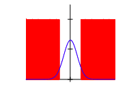
Probability that tunneling is occuring:
\[ 2 \int_{1}^{ \infty} P (x, \beta ) dx = 0.1 \nonumber \]
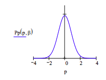
Calculate and display the momentum distribution function:
\[ Pp (p, \beta ) = \int_{- \infty}^{ \infty} W(x, p, \beta ) dx \nonumber \]
Display the Wigner distribution function:
N = 60 i = 0 .. N xi = \( -3 + \frac{6j}{N}\) j = ) .. N pj = \( -5 + \frac{10j}{N}\) Wigneri,j = W(xi, pj, \( \beta\)