Radial and Angular Parts of Atomic Orbitals
- Page ID
- 1712
\( \newcommand{\vecs}[1]{\overset { \scriptstyle \rightharpoonup} {\mathbf{#1}} } \)
\( \newcommand{\vecd}[1]{\overset{-\!-\!\rightharpoonup}{\vphantom{a}\smash {#1}}} \)
\( \newcommand{\dsum}{\displaystyle\sum\limits} \)
\( \newcommand{\dint}{\displaystyle\int\limits} \)
\( \newcommand{\dlim}{\displaystyle\lim\limits} \)
\( \newcommand{\id}{\mathrm{id}}\) \( \newcommand{\Span}{\mathrm{span}}\)
( \newcommand{\kernel}{\mathrm{null}\,}\) \( \newcommand{\range}{\mathrm{range}\,}\)
\( \newcommand{\RealPart}{\mathrm{Re}}\) \( \newcommand{\ImaginaryPart}{\mathrm{Im}}\)
\( \newcommand{\Argument}{\mathrm{Arg}}\) \( \newcommand{\norm}[1]{\| #1 \|}\)
\( \newcommand{\inner}[2]{\langle #1, #2 \rangle}\)
\( \newcommand{\Span}{\mathrm{span}}\)
\( \newcommand{\id}{\mathrm{id}}\)
\( \newcommand{\Span}{\mathrm{span}}\)
\( \newcommand{\kernel}{\mathrm{null}\,}\)
\( \newcommand{\range}{\mathrm{range}\,}\)
\( \newcommand{\RealPart}{\mathrm{Re}}\)
\( \newcommand{\ImaginaryPart}{\mathrm{Im}}\)
\( \newcommand{\Argument}{\mathrm{Arg}}\)
\( \newcommand{\norm}[1]{\| #1 \|}\)
\( \newcommand{\inner}[2]{\langle #1, #2 \rangle}\)
\( \newcommand{\Span}{\mathrm{span}}\) \( \newcommand{\AA}{\unicode[.8,0]{x212B}}\)
\( \newcommand{\vectorA}[1]{\vec{#1}} % arrow\)
\( \newcommand{\vectorAt}[1]{\vec{\text{#1}}} % arrow\)
\( \newcommand{\vectorB}[1]{\overset { \scriptstyle \rightharpoonup} {\mathbf{#1}} } \)
\( \newcommand{\vectorC}[1]{\textbf{#1}} \)
\( \newcommand{\vectorD}[1]{\overrightarrow{#1}} \)
\( \newcommand{\vectorDt}[1]{\overrightarrow{\text{#1}}} \)
\( \newcommand{\vectE}[1]{\overset{-\!-\!\rightharpoonup}{\vphantom{a}\smash{\mathbf {#1}}}} \)
\( \newcommand{\vecs}[1]{\overset { \scriptstyle \rightharpoonup} {\mathbf{#1}} } \)
\(\newcommand{\longvect}{\overrightarrow}\)
\( \newcommand{\vecd}[1]{\overset{-\!-\!\rightharpoonup}{\vphantom{a}\smash {#1}}} \)
\(\newcommand{\avec}{\mathbf a}\) \(\newcommand{\bvec}{\mathbf b}\) \(\newcommand{\cvec}{\mathbf c}\) \(\newcommand{\dvec}{\mathbf d}\) \(\newcommand{\dtil}{\widetilde{\mathbf d}}\) \(\newcommand{\evec}{\mathbf e}\) \(\newcommand{\fvec}{\mathbf f}\) \(\newcommand{\nvec}{\mathbf n}\) \(\newcommand{\pvec}{\mathbf p}\) \(\newcommand{\qvec}{\mathbf q}\) \(\newcommand{\svec}{\mathbf s}\) \(\newcommand{\tvec}{\mathbf t}\) \(\newcommand{\uvec}{\mathbf u}\) \(\newcommand{\vvec}{\mathbf v}\) \(\newcommand{\wvec}{\mathbf w}\) \(\newcommand{\xvec}{\mathbf x}\) \(\newcommand{\yvec}{\mathbf y}\) \(\newcommand{\zvec}{\mathbf z}\) \(\newcommand{\rvec}{\mathbf r}\) \(\newcommand{\mvec}{\mathbf m}\) \(\newcommand{\zerovec}{\mathbf 0}\) \(\newcommand{\onevec}{\mathbf 1}\) \(\newcommand{\real}{\mathbb R}\) \(\newcommand{\twovec}[2]{\left[\begin{array}{r}#1 \\ #2 \end{array}\right]}\) \(\newcommand{\ctwovec}[2]{\left[\begin{array}{c}#1 \\ #2 \end{array}\right]}\) \(\newcommand{\threevec}[3]{\left[\begin{array}{r}#1 \\ #2 \\ #3 \end{array}\right]}\) \(\newcommand{\cthreevec}[3]{\left[\begin{array}{c}#1 \\ #2 \\ #3 \end{array}\right]}\) \(\newcommand{\fourvec}[4]{\left[\begin{array}{r}#1 \\ #2 \\ #3 \\ #4 \end{array}\right]}\) \(\newcommand{\cfourvec}[4]{\left[\begin{array}{c}#1 \\ #2 \\ #3 \\ #4 \end{array}\right]}\) \(\newcommand{\fivevec}[5]{\left[\begin{array}{r}#1 \\ #2 \\ #3 \\ #4 \\ #5 \\ \end{array}\right]}\) \(\newcommand{\cfivevec}[5]{\left[\begin{array}{c}#1 \\ #2 \\ #3 \\ #4 \\ #5 \\ \end{array}\right]}\) \(\newcommand{\mattwo}[4]{\left[\begin{array}{rr}#1 \amp #2 \\ #3 \amp #4 \\ \end{array}\right]}\) \(\newcommand{\laspan}[1]{\text{Span}\{#1\}}\) \(\newcommand{\bcal}{\cal B}\) \(\newcommand{\ccal}{\cal C}\) \(\newcommand{\scal}{\cal S}\) \(\newcommand{\wcal}{\cal W}\) \(\newcommand{\ecal}{\cal E}\) \(\newcommand{\coords}[2]{\left\{#1\right\}_{#2}}\) \(\newcommand{\gray}[1]{\color{gray}{#1}}\) \(\newcommand{\lgray}[1]{\color{lightgray}{#1}}\) \(\newcommand{\rank}{\operatorname{rank}}\) \(\newcommand{\row}{\text{Row}}\) \(\newcommand{\col}{\text{Col}}\) \(\renewcommand{\row}{\text{Row}}\) \(\newcommand{\nul}{\text{Nul}}\) \(\newcommand{\var}{\text{Var}}\) \(\newcommand{\corr}{\text{corr}}\) \(\newcommand{\len}[1]{\left|#1\right|}\) \(\newcommand{\bbar}{\overline{\bvec}}\) \(\newcommand{\bhat}{\widehat{\bvec}}\) \(\newcommand{\bperp}{\bvec^\perp}\) \(\newcommand{\xhat}{\widehat{\xvec}}\) \(\newcommand{\vhat}{\widehat{\vvec}}\) \(\newcommand{\uhat}{\widehat{\uvec}}\) \(\newcommand{\what}{\widehat{\wvec}}\) \(\newcommand{\Sighat}{\widehat{\Sigma}}\) \(\newcommand{\lt}{<}\) \(\newcommand{\gt}{>}\) \(\newcommand{\amp}{&}\) \(\definecolor{fillinmathshade}{gray}{0.9}\)The solutions to Schrödinger's equation for atomic orbitals can be expressed in terms of spherical coordinates: \(r\), \(\theta\), and \(\phi\). For a point \((r, \theta, \phi)\), the variable \(r\) represents the distance from the center of the nucleus, \(\theta\) represents the angle to the positive z-axis, and \(\phi\) represents the angle to the positive x-axis in the xy-plane.
Separation of Variables
Because the atomic orbitals are described with a time-independent potential V, Schrödinger’s equation can be solved using the technique of separation of variables, so that any wavefunction has the form:
\(\Psi(r,\theta,\phi) = R(r) Y(\theta,\phi)\)
where \(R(r)\) is the radial wavefunction and \(Y(\theta,\phi)\) is the angular wavefunction:
\(Y(\theta,\phi) = \Theta(\theta) \; \; \Phi(\phi)\)
Each set of quantum numbers, (\(n\), \(l\), \(m_l\)), describes a different wave function. The radial wave function is only dependent on \(n\) and \(l\), while the angular wavefunction is only dependent on \(l\) and \(m_l\). So a particular orbital solution can be written as:
\(\Psi_{n,l,m_l}(r,\theta,\phi) = {R}_{n,l}(r) Y_{l,m_l}(\theta,\phi)\)
Where
\(n = 1, 2, 3, …\)
\(l = 0, 1, …, n-1\)
\(m_l = -l, … , -2, -1, 0, +1, +2, …, l\)
Nodes
A wave function node occurs at points where the wave function is zero and changes signs. The electron has zero probability of being located at a node.
Because of the separation of variables for an electron orbital, the wave function will be zero when any one of its component functions is zero. When \(R(r)\) is zero, the node consists of a sphere. When \(\Theta(\theta)\) is zero, the node consists of a cone with the z-axis as its axis and apex at the origin. In the special case \(\Theta(\pi/2)\) = 0, the cone is flattened to be the x-y plane. When \(\Phi(\phi)\) is zero, the node consists of a plane through the z-axis.
Bonding and sign of wave function
The shape and extent of an orbital only depends on the square of the magnitude of the wave function. However, when considering how bonding between atoms might take place, the signs of the wave functions are important. As a general rule a bond is stronger, i.e. it has lower energy, when the orbitals of the shared electrons have their wavefunctions match positive to positive and negative to negative. Another way of expressing this is that the bond is stronger when the wave functions constructively interfere with each other. When the orbitals overlap so that the wave functions match positive to negative, the bond will be weaker or may not form at all.
Radial wavefunctions
The radial wavefunctions are of the general form:
\(R(r) = N \; p(r) \; e^{-kr}\)
Where
- \(N\) is a positive normalizing constant
- \(p(r)\) is a polynomial in \(r\)
- \(k\) is a positive constant
The exponential factor is always positive, so the nodes and sign of \(R(r)\) depends on the behavior of \(p(r)\). Because the exponential factor has a negative sign in the exponent, \(R(r)\) will approach 0 as \(r\) goes to infinity.
\(\Psi^2\) quantifies the probability of the electron being at a particular point. The probability distribution, \(P(r)\) is the probability that the electron will be at any point that is \(r\) distance from the nucleus. For any type of orbital, since \(\Psi_{n,0,0}\) is separable into radial and angular components that are each appropriately normalized, and a sphere of radius r has area proportional to \(r^2\), we have:
\(P(r) = r^2R^2(r)\)
Angular wavefunctions
The angular wave function \(Y(\theta,\phi)\)does much to give an orbital its distinctive shape. \(Y(\theta,\phi)\) is typically normalized so the the integral of \(Y^2(\theta,\phi)\) over the unit sphere is equal to one. In this case, \(Y^2(\theta,\phi)\) serves as a probability function. The probability function can be interpreted as the probability that the electron will be found on the ray emitting from the origin that is at angles \((\theta,\phi)\) from the axes. The probability function can also be interpreted as the probability distribution of the electron being at position \((\theta,\phi)\) on a sphere of radius r, given that it is r distance from the nucleus.
The angular wave functions for a hydrogen atom, \(Y_{l,m_l}(\theta,\phi)\) are also the wavefunction solutions to Schrödinger’s equation for a rigid rotor consisting of two bodies, for example a diatomic molecule.
Hydrogen Atom
The simplest case to consider is the hydrogen atom, with one positively charged proton in the nucleus and just one negatively charged electron orbiting around the nucleus. It is important to understand the orbitals of hydrogen, not only because hydrogen is an important element, but also because they serve as building blocks for understanding the orbitals of other atoms.
s Orbitals
The hydrogen s orbitals correspond to \(l=0\) and only allow \(m_l = 0\). In this case, the solution for the angular wavefunction, \(Y_{0,0}(\theta,\phi)\) is a constant. As a result, the \(\Psi_{n,0,0}(r,\theta,\phi)\) wavefunctions only depend on \(r\) and the s orbitals are all spherical in shape.
Because \(\Psi_{n,0,0}\) depends only on r, the probability distribution function of the electron:
\(\Psi^2_{n,0,0}(r,\theta,\phi) = \dfrac{1}{4\pi}R^2_{n,0}(r)\)
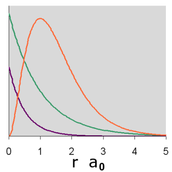
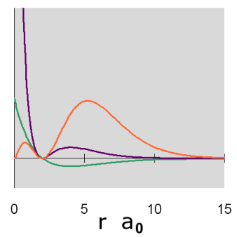
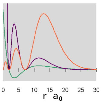
Graphs of the three functions, \(R(r)\) in green, \(R^2(r)\) in purple and \(P(r)\) in orange are given below for n = 1, 2, and 3. The graph of the functions have been variously scaled along the vertical axis to allow an easy comparison of their shapes and where they are zero, positive and negative. The vertical scales for different functions, either within or between diagrams, are not necessarily the same.
In addition, a cross-section contour diagram is given for each of the three orbitals. These contour diagrams indicate the physical shape and size of the orbitals and where the probabilities are concentrated. An electron will be in the most-likely-10% (purple) regions 10% of the time, and it will be in the most-likely-50% regions (including the most-likely-10% regions, dark blue and purple) 50% of the time. Nodes are shown in orange in the contour diagrams. In all of these contour diagrams, the x-axis is horizontal, the z-axis is vertical, and the y-axis comes out of the diagram. The actual 3-dimensional orbital shape is obtained by rotating the 2-dimensional cross-section about the axis of symmetry, which is shown as a blue dashed line. The contour diagrams also indicate for regions that are separated by nodes, whether the wave function is positive (+) or negative (-) in that region. In order for the wave function to change sign, one must cross a node.
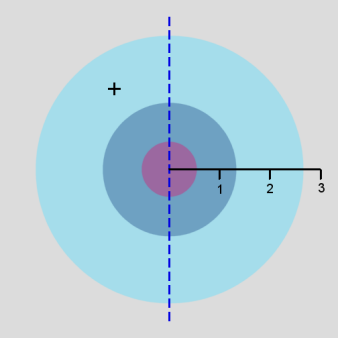
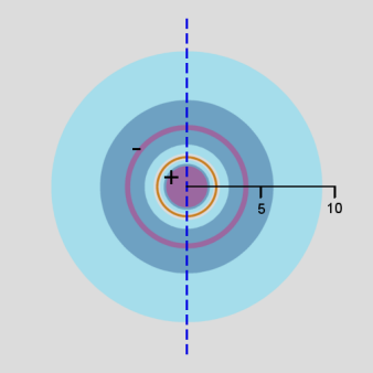
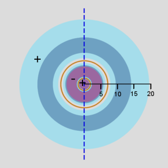
From these diagrams, we see that the 1s orbital does not have any nodes, the 2s orbital has one node, and the 3s orbital has 2 nodes.
Because for the s orbitals, \(\Psi^2 = R^2(r)\), it is interesting to compare the \(R^2(r)\) graphs and the \(P(r)\) graphs. By comparing maximum values, in the 1s orbital, the \(R^2(r)\) graph shows that the most likely place for the electron is at the nucleus, but the \(P(r)\) graph shows that the most likely radius for the electron is at \(a_0\), the Bohr radius. Similarly, for the other s orbitals, the one place the electron is most likely to be is at the nucleus, but the most likely radius for the electron to be at is outside the outermost node. Something that is not readily apparent from these diagrams is that the average radius for the 1s, 2s, and 3s orbitals is 1.5 a0, 6 a0, and 13.5 a0, forming ratios of 1:4:9. In other words, the average radius is proportional to \(n^2\).
p orbitals
The hydrogen p orbitals correspond to l = 1 when n ? 2 and allow ml = -1, 0, or +1. The diagrams below describe the wave function for ml = 0. The angular wave function \(Y_{1,0}(\theta,\phi) = cos\;\theta\) only depends on \(\theta\). Below, the angular wavefunction shown with a node at \(\theta = \pi/2\).
The radial wavefunctions and orbital contour diagrams for the p orbitals with n = 2 and 3 are:
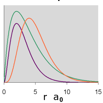
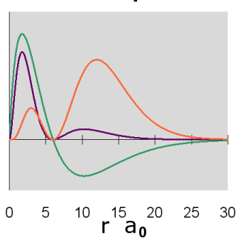
Figure \(\PageIndex{8}\): 3p Orbitals radial diagram
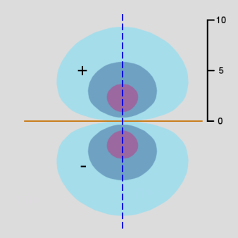
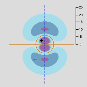
Figure \(\PageIndex{10}\): 3p Orbitals contour diagram
As in the case of the s orbitals, the actual 3-dimensional p orbital shape is obtained by rotating the 2-dimensional cross-sections about the axis of symmetry, which is shown as a blue dashed line.
The p orbitals display their distinctive dumbbell shape. The angular wave function creates a nodal plane (the horizontal line in the cross-section diagram) in the x-y plane. In addition, the 3p radial wavefunction creates a spherical node (the circular node in the cross-section diagram) at r = 6 a0. For \(m_l = 0\), the axis of symmetry is along the z axis.
The wavefunctions for ml = +1 and -1 can be represented in different ways. For ease of computation, they are often represented as real-valued functions. In this case, the orbitals have the same shape and size as \(m_l = 0\), except that they are oriented in a different direction: the axis of symmetry is along the x axis with the nodal plane in the y-z plane or the axis of symmetry is along the y-axis with the nodal plane in the x-z plane. These correspond to wavefunctions that are the sum and the difference of the two ml = +1 and -1 wavefunctions
\[\psi_{x}= \psi_{m_j=+1} + \psi_{m_j=-1} \notag \]
\[\psi_{y}= \psi_{m_j=+1} - \psi_{m_j=-1} \notag \]
the \(\psi_{z}\) wavefunction has a magnetic quantum number of ml =0, but the \(\psi_{x}\) and \(\psi_{y}\) are mixtures of the wavefunctions corresponding to ml = +1 and -1 and do not have unique magnetic quantum numbers.
d Orbitals
The hydrogen d orbitals correspond to l = 2 when n = 3 and allow ml = -2, -1, 0, +1, or +2. There are two basic shapes of d orbitals, depending on the form of the angular wave function.
The first shape of a d orbital corresponds to ml = 0. In this case, \(Y_{2,0}(\theta,\phi)\) only depends on \(\theta\). The graphs of the angular wavefunction, and for \(n = 3\), the radial wave function and orbital contour diagram are as follows:
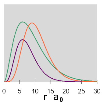

Figure \(\PageIndex{12}\): 3d orbital, ml = 0 Contour Diagram
As in the case of the s and p orbitals, the actual 3-dimensional d orbital shape is obtained by rotating the 2-dimensional cross-section about the axis of symmetry, which is shown as a blue dashed line.
This first d orbital shape displays a dumbbell shape along the z axis, but it is surrounded in the middle by a doughnut (corresponding to the regions where the wavefunction is negative). The angular wave function creates nodes which are cones that open at about 54.7 degrees to the z-axis. At n=3, the radial wave function does not have any nodes.
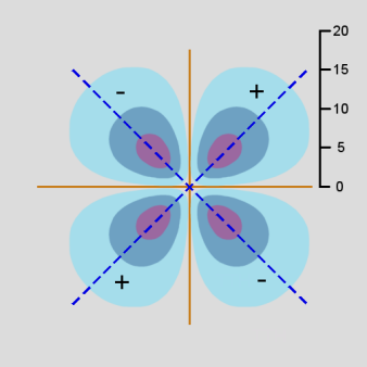
The second d orbital shape is illustrated for ml = +1 and n = 3. In this case, \(Y_{2,1}(\theta,\phi)\) depends on both \(\theta\) and \(\phi\), and can be shown as a surface curving over and under a rectangular domain. As a result, separate diagrams are shown for \(Y_{2,1}(\theta,\phi)\) on the left and \(Y^2_{2,1}(\theta,\phi)\) on the right.
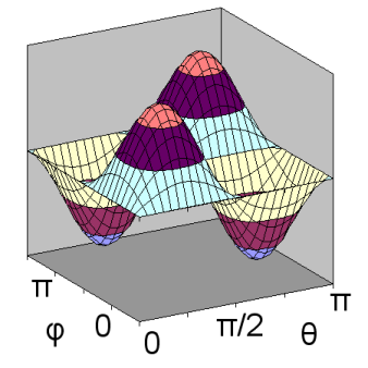
ml = +1: \(Y_{2,1}(\theta,\phi)\)
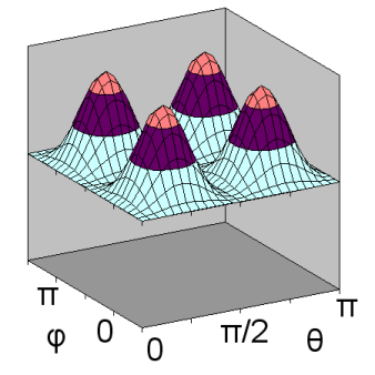
Figure \(\PageIndex{15}\): 3d orbital,
ml = +1: \(Y^2_{2,1}(\theta,\phi)\)
Unlike previous orbital diagrams, this contour diagram indicates more than one axis of symmetry. Each axis of symmetry is at 45 degrees to the x- and z-axis. Each axis of symmetry only applies to the region surrounding it and bounded by nodes. Each of the four arms of the contour is rotated about its axis of symmetry to produce the 3-dimensional shape. However, the rotation is a non-standard rotation, producing only radial symmetry about the axis, not circular symmetry as was the case with other orbitals. This produces a double dumbell shape, with nodes in the x-y plane and the y-z plane.
Similar to the p orbitals, the wavefunctions for ml=+2, -1, and -2 can be represented as real-valued functions that have the same shape as for ml=+1, just oriented in different directions. In two cases, the shape is re-oriented so the the axes of symmetry are in the x-y plane or in the z-y plane. In both of those cases, the axes of symmetry are at 45 degrees to their respective coordinate axes, just as with ml=+1. For the third and final case, the orbital shape is re-oriented so the axes of symmetry are in the x-y plane, but also laying along the x and y axes.
It is often the case that the orbitals in the d subshell corresponding to the magnetic quantum numbers ml = ±1 and ml = ±2 are, as for the \(\psi_{x}\) and \(\psi_{y}\) orbitals, represented as sums and differences of the wavefunctions corresponding to ml = ±1 and ml = ±2. This, as for the p orbitals, better represents the spatial orientation of bonds formed with these orbitals.
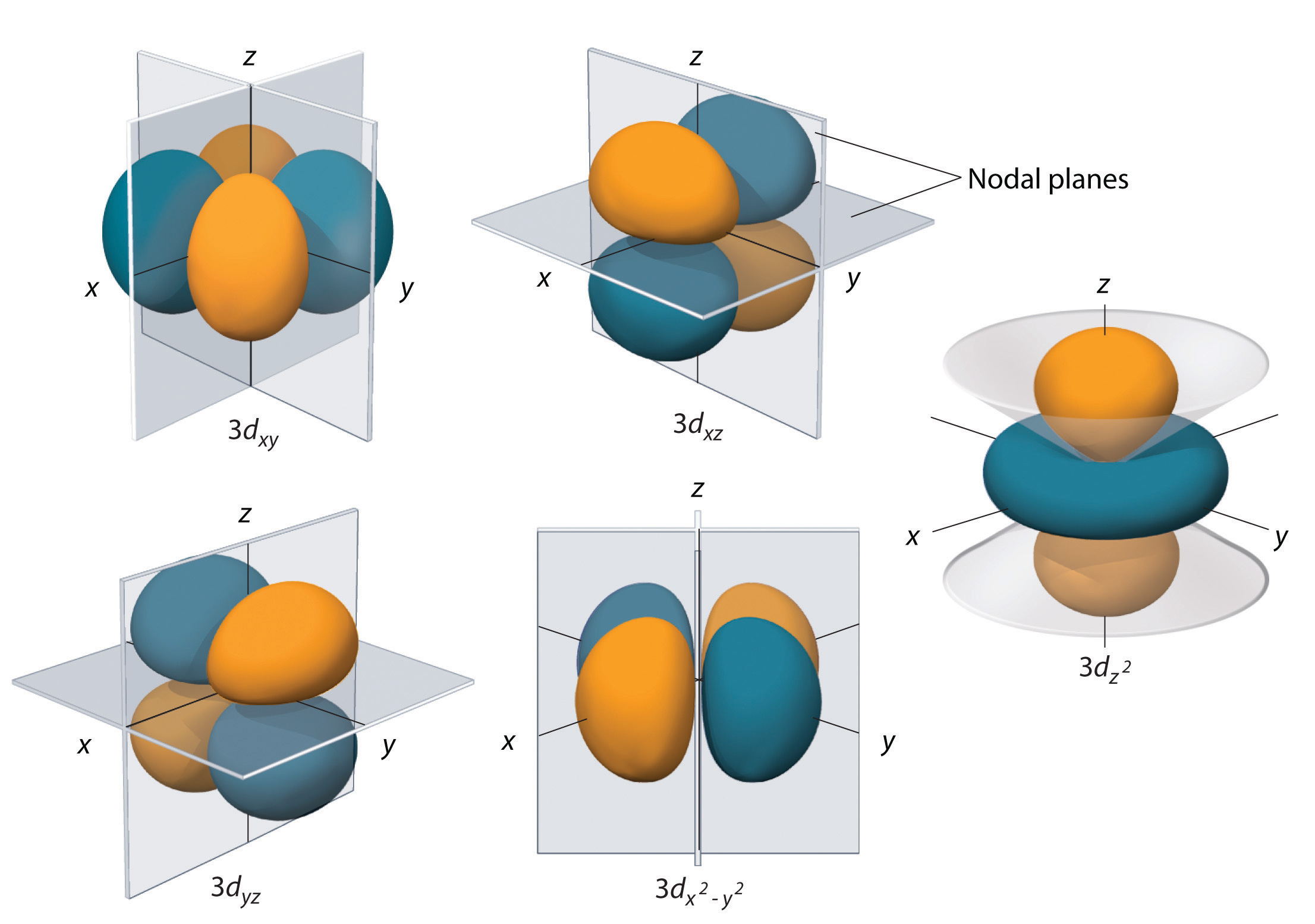
The orbitals dxz and dyz are sums and differences of the two orbitals with ml = ±1 and lie in the xz and yz planes. ml = ±2 similarly corresponds to dxy and dx2 − y2; both lie in the xy plane. ml = 0 is the dz2 orbital, which is oriented along the z-axis.
Hydrogenic Orbitals
Hydrogenic atoms are atoms that only have one electron orbiting around the nucleus, even though the nucleus may have more than one proton and one or more neutrons. In this case, the electron has the same orbitals as the hydrogen atom, except that they are scaled by a factor of 1/Z. Z is the atomic number of the atom, the number of protons in the nucleus. The increased number of positively charged protons shrinks the size of the orbitals.
Thus, the same graphs for hydrogen above apply to hydrogenic atoms, except that instead of expressing the radius in units of a0, the radius is expressed in units of a0/Z. Correspondingly, the  values have to be renormalized by a factor of (Z/a0)3/2. So a He+ atom has orbitals that are the same shape but half the size of the corresponding hydrogen orbitals and a Li2+ atom has orbitals that are the same shape but one third the size of the corresponding hydrogen orbitals.
References
- Atkins, P., & de Paula, J. (2006). Physical Chemistry for the Life Sciences. New York: W. H. Freeman and Company.
- Ladd, M. (1998). Introduction to Physical Chemistry (3rd ed). Cambridge, UK: Cambridge University Press.
- McMahon, D. (2005). Quantum Mechanics Demystified. NewYork: McGraw-Hill Professional.
- McQuarrie, D. A., & Simon, J. D. (1997). Physical Chemistry: A molecular approach. Sausalito, CA: University Science Books.
Contributors and Attributions
- Thanh Hua

