s Atomic Orbitals
- Page ID
- 1637
\( \newcommand{\vecs}[1]{\overset { \scriptstyle \rightharpoonup} {\mathbf{#1}} } \)
\( \newcommand{\vecd}[1]{\overset{-\!-\!\rightharpoonup}{\vphantom{a}\smash {#1}}} \)
\( \newcommand{\dsum}{\displaystyle\sum\limits} \)
\( \newcommand{\dint}{\displaystyle\int\limits} \)
\( \newcommand{\dlim}{\displaystyle\lim\limits} \)
\( \newcommand{\id}{\mathrm{id}}\) \( \newcommand{\Span}{\mathrm{span}}\)
( \newcommand{\kernel}{\mathrm{null}\,}\) \( \newcommand{\range}{\mathrm{range}\,}\)
\( \newcommand{\RealPart}{\mathrm{Re}}\) \( \newcommand{\ImaginaryPart}{\mathrm{Im}}\)
\( \newcommand{\Argument}{\mathrm{Arg}}\) \( \newcommand{\norm}[1]{\| #1 \|}\)
\( \newcommand{\inner}[2]{\langle #1, #2 \rangle}\)
\( \newcommand{\Span}{\mathrm{span}}\)
\( \newcommand{\id}{\mathrm{id}}\)
\( \newcommand{\Span}{\mathrm{span}}\)
\( \newcommand{\kernel}{\mathrm{null}\,}\)
\( \newcommand{\range}{\mathrm{range}\,}\)
\( \newcommand{\RealPart}{\mathrm{Re}}\)
\( \newcommand{\ImaginaryPart}{\mathrm{Im}}\)
\( \newcommand{\Argument}{\mathrm{Arg}}\)
\( \newcommand{\norm}[1]{\| #1 \|}\)
\( \newcommand{\inner}[2]{\langle #1, #2 \rangle}\)
\( \newcommand{\Span}{\mathrm{span}}\) \( \newcommand{\AA}{\unicode[.8,0]{x212B}}\)
\( \newcommand{\vectorA}[1]{\vec{#1}} % arrow\)
\( \newcommand{\vectorAt}[1]{\vec{\text{#1}}} % arrow\)
\( \newcommand{\vectorB}[1]{\overset { \scriptstyle \rightharpoonup} {\mathbf{#1}} } \)
\( \newcommand{\vectorC}[1]{\textbf{#1}} \)
\( \newcommand{\vectorD}[1]{\overrightarrow{#1}} \)
\( \newcommand{\vectorDt}[1]{\overrightarrow{\text{#1}}} \)
\( \newcommand{\vectE}[1]{\overset{-\!-\!\rightharpoonup}{\vphantom{a}\smash{\mathbf {#1}}}} \)
\( \newcommand{\vecs}[1]{\overset { \scriptstyle \rightharpoonup} {\mathbf{#1}} } \)
\(\newcommand{\longvect}{\overrightarrow}\)
\( \newcommand{\vecd}[1]{\overset{-\!-\!\rightharpoonup}{\vphantom{a}\smash {#1}}} \)
\(\newcommand{\avec}{\mathbf a}\) \(\newcommand{\bvec}{\mathbf b}\) \(\newcommand{\cvec}{\mathbf c}\) \(\newcommand{\dvec}{\mathbf d}\) \(\newcommand{\dtil}{\widetilde{\mathbf d}}\) \(\newcommand{\evec}{\mathbf e}\) \(\newcommand{\fvec}{\mathbf f}\) \(\newcommand{\nvec}{\mathbf n}\) \(\newcommand{\pvec}{\mathbf p}\) \(\newcommand{\qvec}{\mathbf q}\) \(\newcommand{\svec}{\mathbf s}\) \(\newcommand{\tvec}{\mathbf t}\) \(\newcommand{\uvec}{\mathbf u}\) \(\newcommand{\vvec}{\mathbf v}\) \(\newcommand{\wvec}{\mathbf w}\) \(\newcommand{\xvec}{\mathbf x}\) \(\newcommand{\yvec}{\mathbf y}\) \(\newcommand{\zvec}{\mathbf z}\) \(\newcommand{\rvec}{\mathbf r}\) \(\newcommand{\mvec}{\mathbf m}\) \(\newcommand{\zerovec}{\mathbf 0}\) \(\newcommand{\onevec}{\mathbf 1}\) \(\newcommand{\real}{\mathbb R}\) \(\newcommand{\twovec}[2]{\left[\begin{array}{r}#1 \\ #2 \end{array}\right]}\) \(\newcommand{\ctwovec}[2]{\left[\begin{array}{c}#1 \\ #2 \end{array}\right]}\) \(\newcommand{\threevec}[3]{\left[\begin{array}{r}#1 \\ #2 \\ #3 \end{array}\right]}\) \(\newcommand{\cthreevec}[3]{\left[\begin{array}{c}#1 \\ #2 \\ #3 \end{array}\right]}\) \(\newcommand{\fourvec}[4]{\left[\begin{array}{r}#1 \\ #2 \\ #3 \\ #4 \end{array}\right]}\) \(\newcommand{\cfourvec}[4]{\left[\begin{array}{c}#1 \\ #2 \\ #3 \\ #4 \end{array}\right]}\) \(\newcommand{\fivevec}[5]{\left[\begin{array}{r}#1 \\ #2 \\ #3 \\ #4 \\ #5 \\ \end{array}\right]}\) \(\newcommand{\cfivevec}[5]{\left[\begin{array}{c}#1 \\ #2 \\ #3 \\ #4 \\ #5 \\ \end{array}\right]}\) \(\newcommand{\mattwo}[4]{\left[\begin{array}{rr}#1 \amp #2 \\ #3 \amp #4 \\ \end{array}\right]}\) \(\newcommand{\laspan}[1]{\text{Span}\{#1\}}\) \(\newcommand{\bcal}{\cal B}\) \(\newcommand{\ccal}{\cal C}\) \(\newcommand{\scal}{\cal S}\) \(\newcommand{\wcal}{\cal W}\) \(\newcommand{\ecal}{\cal E}\) \(\newcommand{\coords}[2]{\left\{#1\right\}_{#2}}\) \(\newcommand{\gray}[1]{\color{gray}{#1}}\) \(\newcommand{\lgray}[1]{\color{lightgray}{#1}}\) \(\newcommand{\rank}{\operatorname{rank}}\) \(\newcommand{\row}{\text{Row}}\) \(\newcommand{\col}{\text{Col}}\) \(\renewcommand{\row}{\text{Row}}\) \(\newcommand{\nul}{\text{Nul}}\) \(\newcommand{\var}{\text{Var}}\) \(\newcommand{\corr}{\text{corr}}\) \(\newcommand{\len}[1]{\left|#1\right|}\) \(\newcommand{\bbar}{\overline{\bvec}}\) \(\newcommand{\bhat}{\widehat{\bvec}}\) \(\newcommand{\bperp}{\bvec^\perp}\) \(\newcommand{\xhat}{\widehat{\xvec}}\) \(\newcommand{\vhat}{\widehat{\vvec}}\) \(\newcommand{\uhat}{\widehat{\uvec}}\) \(\newcommand{\what}{\widehat{\wvec}}\) \(\newcommand{\Sighat}{\widehat{\Sigma}}\) \(\newcommand{\lt}{<}\) \(\newcommand{\gt}{>}\) \(\newcommand{\amp}{&}\) \(\definecolor{fillinmathshade}{gray}{0.9}\)Each n orbital has only one s orbital and therefore two s orbital electrons. Since its angular momentum quantum number(l) is 0, its magnetic quantum number(ml) is also 0. If there is only one electron, the electron can exist in either spin up(ms=1/2) or with spin down(ms=-1/2) configuration; if there are two electrons, they must be one spin up and one spin down.
Basic Description
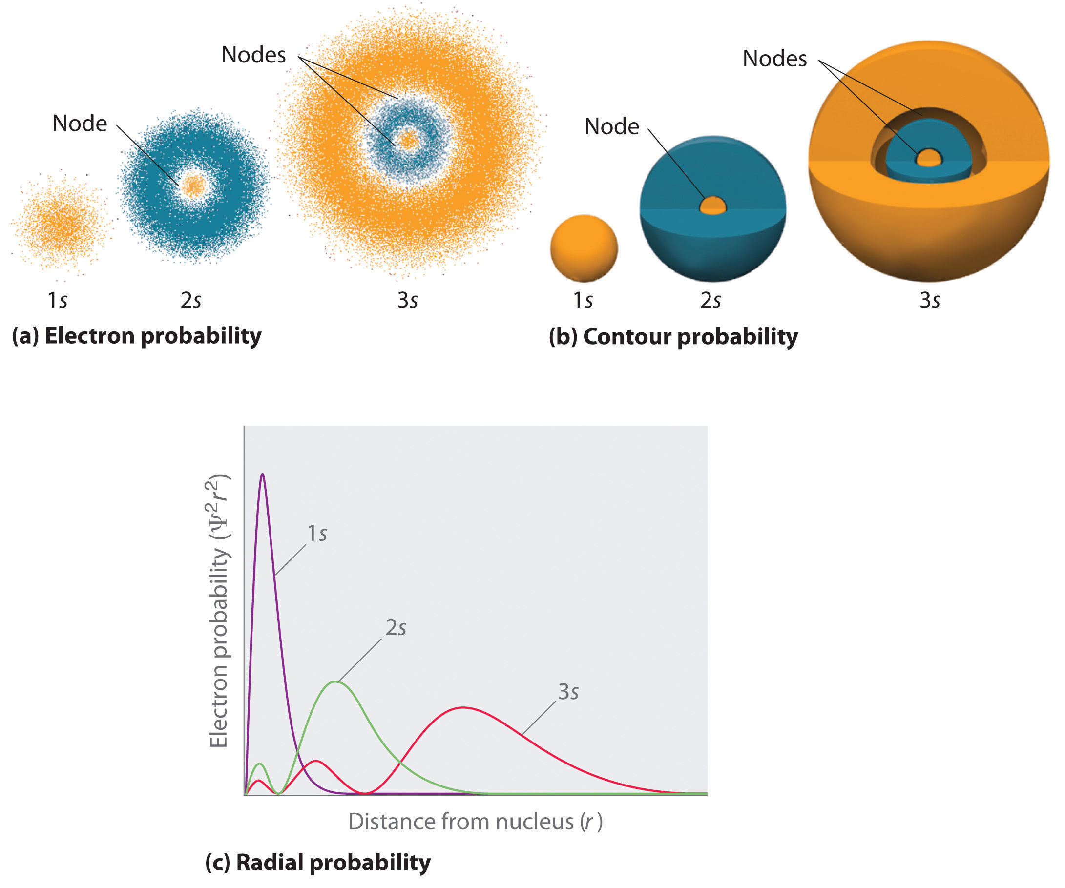
The shape of the s orbital is a sphere; s orbitals are spherically symmetric. The nodes of s orbital is n-1; the angular nodes is l, which is 0 for all s orbitals; the radial nodes is n-l-1, which is n-1 for all s orbitals. Therefore, s orbital only has radial nodes, which are spheres.

If n increases, s orbitals become larger, extending farther from the nucleus. They contain more nodes. This is similar to a standing wave that has regions of significant amplitude separated by nodes, points with zero amplitude. For a given atom, the s orbitals also become higher in energy as n increases because of their increased distance from the nucleus.
Advanced Description
Wavefunction is a mathematical expression that can be used to calculate any property of an atom. In general, wavefunctions depend on both time and position. For atoms, solutions to the Schrödinger equation correspond to arrangements of the electrons, which, if left alone, remain unchanged and are thus only functions of position. S orbitals only have angular wavefunctions, \(Y^{m_J}_J (\theta , \varphi)\) = \(\dfrac {1}{\sqrt {4 \pi}}\), because all s orbitals are l = 0 and therefore ml=0. S orbitals have different radial wavefunctions; for example, for n=1 to n=3, they are R1,0(r) = \(2 \left (\dfrac {Z}{a_0} \right )^{3/2} e^{-\rho}\), R2,0(r) = \( \dfrac {1}{2 \sqrt {2}}\left (\dfrac {Z}{a_0} \right )^{3/2} (2 - \rho) e^{-\rho/2}\), and R3,0(r) = \( \dfrac {1}{81 \sqrt {3}}\left (\dfrac {Z}{a_0} \right )^{3/2} (27 - 18 \rho + 2\rho ^2) e^{-\rho/3}\). Their complete wave functions are \(\psi_{100} = \dfrac {1}{\sqrt {\pi}} \left(\dfrac {Z}{a_0}\right)^{\frac {3}{2}} e^{-\rho}\), \(\psi_{200} = \dfrac {1}{\sqrt {32\pi}} \left(\dfrac {Z}{a_0}\right)^{\frac {3}{2}} (2-\rho)e^{\dfrac {-\rho}{2}}\), and \(\psi_{300} = \dfrac {1}{81\sqrt {3\pi}} \left(\dfrac {Z}{a_0}\right)^{\frac {3}{2}} (27-18\rho +2\rho^2)e^{-\rho/3}\) (\(\rho = \dfrac {Zr}{a_0}\), where \(a_0\) is the Bohr radius and r is the radial variable).
Wavefunctions for each atom have some properties that are exact, for example each wavefunction describes an electron in quantum state with a specific energy.
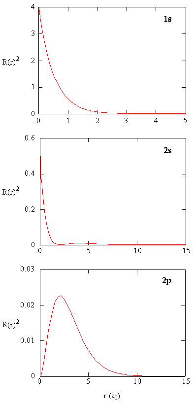
Radial Probability density is the probability density for the electron to be at a point located the distance r from the proton. Radial probability densities for three types of atomic orbitals are plotted below.

S orbitals' radial probability densities at 0 are completely different from p orbitas'.
Radial Probability distribution is the probability density for an electron to be found anywhere on the surface of a sphere located a distance \(r\) from the proton. The area of a spherical surface is \(4 \pi r^2\) (The graph is showed at basic description part).

