6.2.3.4: The Arrhenius Law - Arrhenius Plots
- Page ID
- 1447
\( \newcommand{\vecs}[1]{\overset { \scriptstyle \rightharpoonup} {\mathbf{#1}} } \)
\( \newcommand{\vecd}[1]{\overset{-\!-\!\rightharpoonup}{\vphantom{a}\smash {#1}}} \)
\( \newcommand{\dsum}{\displaystyle\sum\limits} \)
\( \newcommand{\dint}{\displaystyle\int\limits} \)
\( \newcommand{\dlim}{\displaystyle\lim\limits} \)
\( \newcommand{\id}{\mathrm{id}}\) \( \newcommand{\Span}{\mathrm{span}}\)
( \newcommand{\kernel}{\mathrm{null}\,}\) \( \newcommand{\range}{\mathrm{range}\,}\)
\( \newcommand{\RealPart}{\mathrm{Re}}\) \( \newcommand{\ImaginaryPart}{\mathrm{Im}}\)
\( \newcommand{\Argument}{\mathrm{Arg}}\) \( \newcommand{\norm}[1]{\| #1 \|}\)
\( \newcommand{\inner}[2]{\langle #1, #2 \rangle}\)
\( \newcommand{\Span}{\mathrm{span}}\)
\( \newcommand{\id}{\mathrm{id}}\)
\( \newcommand{\Span}{\mathrm{span}}\)
\( \newcommand{\kernel}{\mathrm{null}\,}\)
\( \newcommand{\range}{\mathrm{range}\,}\)
\( \newcommand{\RealPart}{\mathrm{Re}}\)
\( \newcommand{\ImaginaryPart}{\mathrm{Im}}\)
\( \newcommand{\Argument}{\mathrm{Arg}}\)
\( \newcommand{\norm}[1]{\| #1 \|}\)
\( \newcommand{\inner}[2]{\langle #1, #2 \rangle}\)
\( \newcommand{\Span}{\mathrm{span}}\) \( \newcommand{\AA}{\unicode[.8,0]{x212B}}\)
\( \newcommand{\vectorA}[1]{\vec{#1}} % arrow\)
\( \newcommand{\vectorAt}[1]{\vec{\text{#1}}} % arrow\)
\( \newcommand{\vectorB}[1]{\overset { \scriptstyle \rightharpoonup} {\mathbf{#1}} } \)
\( \newcommand{\vectorC}[1]{\textbf{#1}} \)
\( \newcommand{\vectorD}[1]{\overrightarrow{#1}} \)
\( \newcommand{\vectorDt}[1]{\overrightarrow{\text{#1}}} \)
\( \newcommand{\vectE}[1]{\overset{-\!-\!\rightharpoonup}{\vphantom{a}\smash{\mathbf {#1}}}} \)
\( \newcommand{\vecs}[1]{\overset { \scriptstyle \rightharpoonup} {\mathbf{#1}} } \)
\( \newcommand{\vecd}[1]{\overset{-\!-\!\rightharpoonup}{\vphantom{a}\smash {#1}}} \)
\(\newcommand{\avec}{\mathbf a}\) \(\newcommand{\bvec}{\mathbf b}\) \(\newcommand{\cvec}{\mathbf c}\) \(\newcommand{\dvec}{\mathbf d}\) \(\newcommand{\dtil}{\widetilde{\mathbf d}}\) \(\newcommand{\evec}{\mathbf e}\) \(\newcommand{\fvec}{\mathbf f}\) \(\newcommand{\nvec}{\mathbf n}\) \(\newcommand{\pvec}{\mathbf p}\) \(\newcommand{\qvec}{\mathbf q}\) \(\newcommand{\svec}{\mathbf s}\) \(\newcommand{\tvec}{\mathbf t}\) \(\newcommand{\uvec}{\mathbf u}\) \(\newcommand{\vvec}{\mathbf v}\) \(\newcommand{\wvec}{\mathbf w}\) \(\newcommand{\xvec}{\mathbf x}\) \(\newcommand{\yvec}{\mathbf y}\) \(\newcommand{\zvec}{\mathbf z}\) \(\newcommand{\rvec}{\mathbf r}\) \(\newcommand{\mvec}{\mathbf m}\) \(\newcommand{\zerovec}{\mathbf 0}\) \(\newcommand{\onevec}{\mathbf 1}\) \(\newcommand{\real}{\mathbb R}\) \(\newcommand{\twovec}[2]{\left[\begin{array}{r}#1 \\ #2 \end{array}\right]}\) \(\newcommand{\ctwovec}[2]{\left[\begin{array}{c}#1 \\ #2 \end{array}\right]}\) \(\newcommand{\threevec}[3]{\left[\begin{array}{r}#1 \\ #2 \\ #3 \end{array}\right]}\) \(\newcommand{\cthreevec}[3]{\left[\begin{array}{c}#1 \\ #2 \\ #3 \end{array}\right]}\) \(\newcommand{\fourvec}[4]{\left[\begin{array}{r}#1 \\ #2 \\ #3 \\ #4 \end{array}\right]}\) \(\newcommand{\cfourvec}[4]{\left[\begin{array}{c}#1 \\ #2 \\ #3 \\ #4 \end{array}\right]}\) \(\newcommand{\fivevec}[5]{\left[\begin{array}{r}#1 \\ #2 \\ #3 \\ #4 \\ #5 \\ \end{array}\right]}\) \(\newcommand{\cfivevec}[5]{\left[\begin{array}{c}#1 \\ #2 \\ #3 \\ #4 \\ #5 \\ \end{array}\right]}\) \(\newcommand{\mattwo}[4]{\left[\begin{array}{rr}#1 \amp #2 \\ #3 \amp #4 \\ \end{array}\right]}\) \(\newcommand{\laspan}[1]{\text{Span}\{#1\}}\) \(\newcommand{\bcal}{\cal B}\) \(\newcommand{\ccal}{\cal C}\) \(\newcommand{\scal}{\cal S}\) \(\newcommand{\wcal}{\cal W}\) \(\newcommand{\ecal}{\cal E}\) \(\newcommand{\coords}[2]{\left\{#1\right\}_{#2}}\) \(\newcommand{\gray}[1]{\color{gray}{#1}}\) \(\newcommand{\lgray}[1]{\color{lightgray}{#1}}\) \(\newcommand{\rank}{\operatorname{rank}}\) \(\newcommand{\row}{\text{Row}}\) \(\newcommand{\col}{\text{Col}}\) \(\renewcommand{\row}{\text{Row}}\) \(\newcommand{\nul}{\text{Nul}}\) \(\newcommand{\var}{\text{Var}}\) \(\newcommand{\corr}{\text{corr}}\) \(\newcommand{\len}[1]{\left|#1\right|}\) \(\newcommand{\bbar}{\overline{\bvec}}\) \(\newcommand{\bhat}{\widehat{\bvec}}\) \(\newcommand{\bperp}{\bvec^\perp}\) \(\newcommand{\xhat}{\widehat{\xvec}}\) \(\newcommand{\vhat}{\widehat{\vvec}}\) \(\newcommand{\uhat}{\widehat{\uvec}}\) \(\newcommand{\what}{\widehat{\wvec}}\) \(\newcommand{\Sighat}{\widehat{\Sigma}}\) \(\newcommand{\lt}{<}\) \(\newcommand{\gt}{>}\) \(\newcommand{\amp}{&}\) \(\definecolor{fillinmathshade}{gray}{0.9}\)In 1889, Svante Arrhenius proposed the Arrhenius equation from his direct observations of the plots of rate constants vs. temperatures:
\[k = Ae^{-\frac{E_a}{RT}} \label{eq1} \]
The activation energy, Ea, is the minimum energy molecules must possess in order to react to form a product. The slope of the Arrhenius plot can be used to find the activation energy. The Arrhenius plot can also be used by extrapolating the line back to the y-intercept to obtain the pre-exponential factor, A. This factor is significant because A=p×Z, where p is a steric factor and Z is the collision frequency. The pre-exponential, or frequency, factor is related to the amount of times molecules will hit in the orientation necessary to cause a reaction. It is important to note that the Arrhenius equation is based on the collision theory. It states that particles must collide with proper orientation and with enough energy. Now that we have obtained the activation energy and pre-exponential factor from the Arrhenius plot, we can solve for the rate constant at any temperature using the Arrhenius equation.
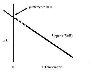
The Arrhenius plot is obtained by plotting the logarithm of the rate constant, k, versus the inverse temperature, 1/T. The resulting negatively-sloped line is useful in finding the missing components of the Arrhenius equation. Extrapolation of the line back to the y-intercept yields the value for ln A. The slope of the line is equal to the negative activation energy divided by the gas constant, R. As a rule of thumb in most biological and chemical reactions, the reaction rate doubles when the temperature increases every 10 degrees Celsius.

Looking at the Arrhenius equation, the denominator of the exponential function contains the gas constant, R, and the temperature, T. This is only the case when dealing with moles of a substance, because R has the units of J/molK. When dealing with molecules of a substance, the gas constant in the dominator of the exponential function of the Arrhenius equation is replaced by the Boltzmann constant, kB. The Boltzmann constant has the units J/K. At room temperature, kBT, is the available energy for a molecule at 25 C or 273K, and is equal to approximately 200 wave numbers.
It is important to note that the decision to use the gas constant or the Boltzmann constant in the Arrhenius equation depends primarily on the canceling of the units. To take the inverse log of a number, the number must be unitless. Therefore all the units in the exponential factor must cancel out. If the activation energy is in terms of joules per moles, then the gas constant should be used in the dominator. However, if the activation energy is in unit of joules per molecule, then the constant, K, should be used.
- Arrhenius Equation per Mole \[k = Ae^{\frac{-E_a}{RT}} \nonumber \]
- Arrhenius Equation per Molecule \[k = Ae^{\frac{-E_a}{KT}} \nonumber \]
"Linearized" Arrhenius Equation
The Arrhenius equation (Equation \ref{eq1}) can be rearranged to deal with specific situations. For example, taking the logarithm of both sides yields the equation above in the form y=-mx+b.
\[\ln k = \dfrac{-E_a}{RT}+\ln A \label{eq2} \]
Then, a plot of \(\ln k\) vs. \(1/T\) and all variables can be found.
- \(y=ln k\)
- \(m=-Ea/RT\)
- \(x=1/T\)
- \(b=\ln A\)
This form of the Arrhenius equation makes it easy to determine the slope and y-intercept from an Arrhenius plot. It is also convenient to note that the above equation shows the connection between temperature and rate constant. As the temperature increases, the rate constant decreases according to the plot. From this connection we can infer that the rate constant is inversely proportional to temperature.
Integrated Form
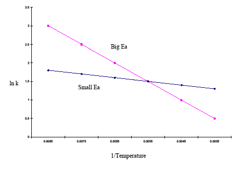
The integrated form of the Arrhenius equation is also useful (Equation \ref{eq3}). This variation of the Arrhenius equation involves the use of two Arrhenius plots constructed on the same graph to determine the activation energy. The above equation, shows temperature's effect on multiple rate constants. This allows easy inference of the rate constants' sensitivity to activation energy and temperature changes. If the activation energy is high for a given temperature range, then the rate constant is highly sensitive; changes in temperature have a significant effect on the rate constant. If the activation energy is low for a given temperature range, then the rate constant is less sensitive, and changes in temperature have little effect on the rate constant. This phenomenon is graphically illustrated in the example below:
| 1/Temp | 0.0085 | 0.0075 | 0.0065 | 0.0055 | 0.0045 | 0.0035 |
|---|---|---|---|---|---|---|
| lnk (large Ea) | 3 | 2.5 | 2 | 1.5 | 1 | 0.5 |
| lnk (small Ea) | 1.8 | 1.7 | 1.6 | 1.5 | 1.4 | 1.3 |

The graph above shows that the plot with the steeper slope has a higher activation energy and the plot with the flatter slope has a smaller activation energy. This means that over the same temperature range, a reaction with a higher activation energy changes more rapidly than a reaction with a lower activation energy.
The Arrhenius plot may become non-linear if steps become rate-limiting at different temperatures. Such an example can be found with Fox and co-workers in 1972 with beta-glycoside transport in E. coli. The differences in the transition temperatures are due to fatty acid composition in cell membranes. The transition state difference is a result of the sharp change of fluidity of the membrane. Another example includes a sudden drop at low 1/T (high temperatures), a result of protein denaturation.
Key Points
- Arrhenius plots show that reaction rates are inversely proportional to temperature changes
- The negative slope from the Arrhenius plot gives the activation energy, Ea: slope = -Ea/R
- Extrapolation of the Arrhenius plot back to the y-intercept gives lnA
- The arrhenius plot shows how activation energy and temperature affect the sensitivity of the reaction rate
Practice Problems
1. T/F The Ea calculated from the Arrhenius equation gives an exact value.
2. Describe the relationship between temperature and Ea and give examples.
3. Using the following information:
A= 1×10¹⁴sec-1
Ea= 75×103 J/mol
R= 8.314 J mol/K
Calculate k at 27° C with proper units.
4. Using information from problem 3, calculate k at 37° C with proper units.
5. Using the integrated equation solve for Ea using:
k1=7.78×10⁻⁷ at T1=273 K
k2=3.46×10⁻⁵ at T2=298 K
Answers
- False: Ea is an average or "apparent" value.
- As the temperature increases, the rate constant decreases when the above equation is plotted. The same is true when the temperature decreases, the rate constant increases. From this connection, the rate constant is inversely proportional to temperature.
- k= 8.727 sec-1
- k=23.02 sec-1
- Ea=1.026×10⁵ J/mol
References
- Alberty, R. A. and R. J. Silbey (1997). Physical chemistry. New York, Wiley.
- Petrucci, R. H., W. S. Harwood, et al. (2002). General chemistry: principles and modern applications. Upper Saddle River, N.J., Prentice Hall.
- Dawber, J. G. and A. T. Moore (1973). Chemistry for the life sciences. London, New York, McGraw-Hill.
- Atkins, P. W. and J. De Paula (2006). Physical chemistry for the life sciences. New York, Oxford University Press; Freeman.
- Stiller, W. (1989). Arrhenius equation and non-equilibrium kinetics: 100 years Arrhenius equation. Leipzig, BSB B.G. Teubner.
- Segel, Irwin H. (1975). Enzyme Kinetics: Behavior and Analysis of Rapid Equilibrium and Steady-State Enzyme Systems. John Wiley and Sons Inc.
Contributors and Attributions
- David Johns and Andra Hutton (UC Davis)

