6.1.5: Introduction
- Page ID
- 9657
\( \newcommand{\vecs}[1]{\overset { \scriptstyle \rightharpoonup} {\mathbf{#1}} } \)
\( \newcommand{\vecd}[1]{\overset{-\!-\!\rightharpoonup}{\vphantom{a}\smash {#1}}} \)
\( \newcommand{\id}{\mathrm{id}}\) \( \newcommand{\Span}{\mathrm{span}}\)
( \newcommand{\kernel}{\mathrm{null}\,}\) \( \newcommand{\range}{\mathrm{range}\,}\)
\( \newcommand{\RealPart}{\mathrm{Re}}\) \( \newcommand{\ImaginaryPart}{\mathrm{Im}}\)
\( \newcommand{\Argument}{\mathrm{Arg}}\) \( \newcommand{\norm}[1]{\| #1 \|}\)
\( \newcommand{\inner}[2]{\langle #1, #2 \rangle}\)
\( \newcommand{\Span}{\mathrm{span}}\)
\( \newcommand{\id}{\mathrm{id}}\)
\( \newcommand{\Span}{\mathrm{span}}\)
\( \newcommand{\kernel}{\mathrm{null}\,}\)
\( \newcommand{\range}{\mathrm{range}\,}\)
\( \newcommand{\RealPart}{\mathrm{Re}}\)
\( \newcommand{\ImaginaryPart}{\mathrm{Im}}\)
\( \newcommand{\Argument}{\mathrm{Arg}}\)
\( \newcommand{\norm}[1]{\| #1 \|}\)
\( \newcommand{\inner}[2]{\langle #1, #2 \rangle}\)
\( \newcommand{\Span}{\mathrm{span}}\) \( \newcommand{\AA}{\unicode[.8,0]{x212B}}\)
\( \newcommand{\vectorA}[1]{\vec{#1}} % arrow\)
\( \newcommand{\vectorAt}[1]{\vec{\text{#1}}} % arrow\)
\( \newcommand{\vectorB}[1]{\overset { \scriptstyle \rightharpoonup} {\mathbf{#1}} } \)
\( \newcommand{\vectorC}[1]{\textbf{#1}} \)
\( \newcommand{\vectorD}[1]{\overrightarrow{#1}} \)
\( \newcommand{\vectorDt}[1]{\overrightarrow{\text{#1}}} \)
\( \newcommand{\vectE}[1]{\overset{-\!-\!\rightharpoonup}{\vphantom{a}\smash{\mathbf {#1}}}} \)
\( \newcommand{\vecs}[1]{\overset { \scriptstyle \rightharpoonup} {\mathbf{#1}} } \)
\( \newcommand{\vecd}[1]{\overset{-\!-\!\rightharpoonup}{\vphantom{a}\smash {#1}}} \)
\(\newcommand{\avec}{\mathbf a}\) \(\newcommand{\bvec}{\mathbf b}\) \(\newcommand{\cvec}{\mathbf c}\) \(\newcommand{\dvec}{\mathbf d}\) \(\newcommand{\dtil}{\widetilde{\mathbf d}}\) \(\newcommand{\evec}{\mathbf e}\) \(\newcommand{\fvec}{\mathbf f}\) \(\newcommand{\nvec}{\mathbf n}\) \(\newcommand{\pvec}{\mathbf p}\) \(\newcommand{\qvec}{\mathbf q}\) \(\newcommand{\svec}{\mathbf s}\) \(\newcommand{\tvec}{\mathbf t}\) \(\newcommand{\uvec}{\mathbf u}\) \(\newcommand{\vvec}{\mathbf v}\) \(\newcommand{\wvec}{\mathbf w}\) \(\newcommand{\xvec}{\mathbf x}\) \(\newcommand{\yvec}{\mathbf y}\) \(\newcommand{\zvec}{\mathbf z}\) \(\newcommand{\rvec}{\mathbf r}\) \(\newcommand{\mvec}{\mathbf m}\) \(\newcommand{\zerovec}{\mathbf 0}\) \(\newcommand{\onevec}{\mathbf 1}\) \(\newcommand{\real}{\mathbb R}\) \(\newcommand{\twovec}[2]{\left[\begin{array}{r}#1 \\ #2 \end{array}\right]}\) \(\newcommand{\ctwovec}[2]{\left[\begin{array}{c}#1 \\ #2 \end{array}\right]}\) \(\newcommand{\threevec}[3]{\left[\begin{array}{r}#1 \\ #2 \\ #3 \end{array}\right]}\) \(\newcommand{\cthreevec}[3]{\left[\begin{array}{c}#1 \\ #2 \\ #3 \end{array}\right]}\) \(\newcommand{\fourvec}[4]{\left[\begin{array}{r}#1 \\ #2 \\ #3 \\ #4 \end{array}\right]}\) \(\newcommand{\cfourvec}[4]{\left[\begin{array}{c}#1 \\ #2 \\ #3 \\ #4 \end{array}\right]}\) \(\newcommand{\fivevec}[5]{\left[\begin{array}{r}#1 \\ #2 \\ #3 \\ #4 \\ #5 \\ \end{array}\right]}\) \(\newcommand{\cfivevec}[5]{\left[\begin{array}{c}#1 \\ #2 \\ #3 \\ #4 \\ #5 \\ \end{array}\right]}\) \(\newcommand{\mattwo}[4]{\left[\begin{array}{rr}#1 \amp #2 \\ #3 \amp #4 \\ \end{array}\right]}\) \(\newcommand{\laspan}[1]{\text{Span}\{#1\}}\) \(\newcommand{\bcal}{\cal B}\) \(\newcommand{\ccal}{\cal C}\) \(\newcommand{\scal}{\cal S}\) \(\newcommand{\wcal}{\cal W}\) \(\newcommand{\ecal}{\cal E}\) \(\newcommand{\coords}[2]{\left\{#1\right\}_{#2}}\) \(\newcommand{\gray}[1]{\color{gray}{#1}}\) \(\newcommand{\lgray}[1]{\color{lightgray}{#1}}\) \(\newcommand{\rank}{\operatorname{rank}}\) \(\newcommand{\row}{\text{Row}}\) \(\newcommand{\col}{\text{Col}}\) \(\renewcommand{\row}{\text{Row}}\) \(\newcommand{\nul}{\text{Nul}}\) \(\newcommand{\var}{\text{Var}}\) \(\newcommand{\corr}{\text{corr}}\) \(\newcommand{\len}[1]{\left|#1\right|}\) \(\newcommand{\bbar}{\overline{\bvec}}\) \(\newcommand{\bhat}{\widehat{\bvec}}\) \(\newcommand{\bperp}{\bvec^\perp}\) \(\newcommand{\xhat}{\widehat{\xvec}}\) \(\newcommand{\vhat}{\widehat{\vvec}}\) \(\newcommand{\uhat}{\widehat{\uvec}}\) \(\newcommand{\what}{\widehat{\wvec}}\) \(\newcommand{\Sighat}{\widehat{\Sigma}}\) \(\newcommand{\lt}{<}\) \(\newcommand{\gt}{>}\) \(\newcommand{\amp}{&}\) \(\definecolor{fillinmathshade}{gray}{0.9}\)Collision Frequency
The rate at which molecules collide which is the frequency of collisions is called the collision frequency, Z, which has units of collisions per unit of time. Given a box of molecules A and B, the collision frequency between molecules A and B is defined by the following equation:
\[Z=N_{A}N_{B}\sigma_{AB}\sqrt{\dfrac{8k_{B}T}{\pi\mu_{AB}}} \nonumber \]
where:
- NA and NB are the numbers of molecules A and B, and is directly related to the concentrations of A and B.
- \(\sqrt{\dfrac{8k_{B}T}{\pi\mu_{AB}}}\) is the mean speed of molecules.
- \(\sigma_{AB}\) is the averaged sum of the collision cross sections of molecules A and B. The collision cross section represents the collision region presented by one molecule to another.
Successful Collisions
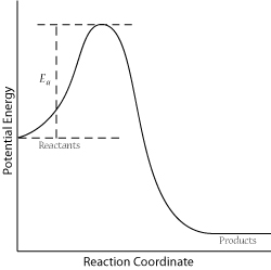
In order for a successful collision to occur, the reactant molecules must collide with enough kinetic energy to break original bonds and form new bonds to become the product molecules. This energy is called the activation energy for the reaction; it is also often referred to as the energy barrier.

The fraction of collisions with enough energy to overcome the activation barrier is given by:
\(f = e^{\frac{-E_a}{RT}}\)
where:
- f is the fraction of collisions with enough energy
- Ea is the activation energy
The fraction of successful collisions is directly proportional to the temperature and inversely proportional to the activation energy.
Putting it all Together
The rate constant of the gas-phase reaction is proportional to the product of the collision frequency and the fraction of successful reactions. As stated above, sufficient kinetic energy is required for a successful reaction; however, they must also collide properly (see below). Compare the following equation to the Arrhenius equation:
\(k = Z\rho{e^{\frac{-E_a}{RT}}}\)
where
- k is the rate constant for the reaction
- ρ is the steric factor. It is the probability of the reactant molecules colliding with the right orientation and positioning to achieve a product with the desirable geometry and stereospecificity. The steric factor is very difficult to assess on paper; it is determined experimentally.
- Zρ is the pre-exponential factor, A, of the Arrhenius equation. In theory, it is the frequency of total collisions that collide with the right orientation. In practice, it is the pre-exponential factor that is directly determined by experiment and then used to calculate the steric factor.
- Ea is activation energy
- T is absolute temperature
- R is gas constant.
Collision Frequency Equation
The collision frequency equation can thus be given as follows:
\[Z = N_A\rho_{AB} \sqrt{\frac{8k_BT}{\pi\mu_{AB}}} \nonumber \]
where:
- NA is number of molecules per unit volume
- kB is Boltzmann's constant
Examples of gas-phase reactions and their steric factors
Reactions with more complex reactants and greater needs for collision orientation specificity, such as that below, have smaller steric factors (and therefore lower chances of success).
\[H_2 + C_2H_4 \rightarrow C_2H_6 \nonumber \]
The opposite holds true for simpler reactions; they have a relatively larger steric factors:
\[H^. + H^. \rightarrow H_2 \nonumber \]
Applications
The collision theory is used to predict the reaction rates for gas-phase reactions. It is a rough approximation due to the complications of the steric factor; furthermore, some of the assumptions do not hold in practical scenarios. For example, in real life molecules are not perfect spheres. Finally, the concepts of collision frequency can be applied in the laboratory:
- The temperature of the environment affects the average speed of molecules. Thus, reactions are heated to increase the reaction rate.
- The initial concentration of reactants is directly proportional to the collision frequency; increasing the initial concentration will speed up the reaction.
Although the collision theory deals with gas-phase reactions, its concepts can also be applied to reactions that take place in solvents; however, the properties of the solvents (for example: solvent cage) will affect the rate of reactions. Ultimately, collision theory illustrates how reactions occur; it can be used to approximate the rate constants of reactions, and its concepts can be directly applied in the laboratory.
References
- Atkins, Peter and Julio de Paula. Physical Chemistry for the Life Sciences. 2006. New York, NY: W.H. Freeman and Company. p.281-3, 290
- Petrucci, R. H., Harwood, W. S., & Herring, F. G. (2002). General Chemistry: Principles and Modern Applications. Upper Saddle River, NJ: Prentice-Hall, Inc. p.597-9

