
Metallic Bonding
- Page ID
- 1989

\( \newcommand{\vecs}[1]{\overset { \scriptstyle \rightharpoonup} {\mathbf{#1}} } \)
\( \newcommand{\vecd}[1]{\overset{-\!-\!\rightharpoonup}{\vphantom{a}\smash {#1}}} \)
\( \newcommand{\dsum}{\displaystyle\sum\limits} \)
\( \newcommand{\dint}{\displaystyle\int\limits} \)
\( \newcommand{\dlim}{\displaystyle\lim\limits} \)
\( \newcommand{\id}{\mathrm{id}}\) \( \newcommand{\Span}{\mathrm{span}}\)
( \newcommand{\kernel}{\mathrm{null}\,}\) \( \newcommand{\range}{\mathrm{range}\,}\)
\( \newcommand{\RealPart}{\mathrm{Re}}\) \( \newcommand{\ImaginaryPart}{\mathrm{Im}}\)
\( \newcommand{\Argument}{\mathrm{Arg}}\) \( \newcommand{\norm}[1]{\| #1 \|}\)
\( \newcommand{\inner}[2]{\langle #1, #2 \rangle}\)
\( \newcommand{\Span}{\mathrm{span}}\)
\( \newcommand{\id}{\mathrm{id}}\)
\( \newcommand{\Span}{\mathrm{span}}\)
\( \newcommand{\kernel}{\mathrm{null}\,}\)
\( \newcommand{\range}{\mathrm{range}\,}\)
\( \newcommand{\RealPart}{\mathrm{Re}}\)
\( \newcommand{\ImaginaryPart}{\mathrm{Im}}\)
\( \newcommand{\Argument}{\mathrm{Arg}}\)
\( \newcommand{\norm}[1]{\| #1 \|}\)
\( \newcommand{\inner}[2]{\langle #1, #2 \rangle}\)
\( \newcommand{\Span}{\mathrm{span}}\) \( \newcommand{\AA}{\unicode[.8,0]{x212B}}\)
\( \newcommand{\vectorA}[1]{\vec{#1}} % arrow\)
\( \newcommand{\vectorAt}[1]{\vec{\text{#1}}} % arrow\)
\( \newcommand{\vectorB}[1]{\overset { \scriptstyle \rightharpoonup} {\mathbf{#1}} } \)
\( \newcommand{\vectorC}[1]{\textbf{#1}} \)
\( \newcommand{\vectorD}[1]{\overrightarrow{#1}} \)
\( \newcommand{\vectorDt}[1]{\overrightarrow{\text{#1}}} \)
\( \newcommand{\vectE}[1]{\overset{-\!-\!\rightharpoonup}{\vphantom{a}\smash{\mathbf {#1}}}} \)
\( \newcommand{\vecs}[1]{\overset { \scriptstyle \rightharpoonup} {\mathbf{#1}} } \)
\(\newcommand{\longvect}{\overrightarrow}\)
\( \newcommand{\vecd}[1]{\overset{-\!-\!\rightharpoonup}{\vphantom{a}\smash {#1}}} \)
\(\newcommand{\avec}{\mathbf a}\) \(\newcommand{\bvec}{\mathbf b}\) \(\newcommand{\cvec}{\mathbf c}\) \(\newcommand{\dvec}{\mathbf d}\) \(\newcommand{\dtil}{\widetilde{\mathbf d}}\) \(\newcommand{\evec}{\mathbf e}\) \(\newcommand{\fvec}{\mathbf f}\) \(\newcommand{\nvec}{\mathbf n}\) \(\newcommand{\pvec}{\mathbf p}\) \(\newcommand{\qvec}{\mathbf q}\) \(\newcommand{\svec}{\mathbf s}\) \(\newcommand{\tvec}{\mathbf t}\) \(\newcommand{\uvec}{\mathbf u}\) \(\newcommand{\vvec}{\mathbf v}\) \(\newcommand{\wvec}{\mathbf w}\) \(\newcommand{\xvec}{\mathbf x}\) \(\newcommand{\yvec}{\mathbf y}\) \(\newcommand{\zvec}{\mathbf z}\) \(\newcommand{\rvec}{\mathbf r}\) \(\newcommand{\mvec}{\mathbf m}\) \(\newcommand{\zerovec}{\mathbf 0}\) \(\newcommand{\onevec}{\mathbf 1}\) \(\newcommand{\real}{\mathbb R}\) \(\newcommand{\twovec}[2]{\left[\begin{array}{r}#1 \\ #2 \end{array}\right]}\) \(\newcommand{\ctwovec}[2]{\left[\begin{array}{c}#1 \\ #2 \end{array}\right]}\) \(\newcommand{\threevec}[3]{\left[\begin{array}{r}#1 \\ #2 \\ #3 \end{array}\right]}\) \(\newcommand{\cthreevec}[3]{\left[\begin{array}{c}#1 \\ #2 \\ #3 \end{array}\right]}\) \(\newcommand{\fourvec}[4]{\left[\begin{array}{r}#1 \\ #2 \\ #3 \\ #4 \end{array}\right]}\) \(\newcommand{\cfourvec}[4]{\left[\begin{array}{c}#1 \\ #2 \\ #3 \\ #4 \end{array}\right]}\) \(\newcommand{\fivevec}[5]{\left[\begin{array}{r}#1 \\ #2 \\ #3 \\ #4 \\ #5 \\ \end{array}\right]}\) \(\newcommand{\cfivevec}[5]{\left[\begin{array}{c}#1 \\ #2 \\ #3 \\ #4 \\ #5 \\ \end{array}\right]}\) \(\newcommand{\mattwo}[4]{\left[\begin{array}{rr}#1 \amp #2 \\ #3 \amp #4 \\ \end{array}\right]}\) \(\newcommand{\laspan}[1]{\text{Span}\{#1\}}\) \(\newcommand{\bcal}{\cal B}\) \(\newcommand{\ccal}{\cal C}\) \(\newcommand{\scal}{\cal S}\) \(\newcommand{\wcal}{\cal W}\) \(\newcommand{\ecal}{\cal E}\) \(\newcommand{\coords}[2]{\left\{#1\right\}_{#2}}\) \(\newcommand{\gray}[1]{\color{gray}{#1}}\) \(\newcommand{\lgray}[1]{\color{lightgray}{#1}}\) \(\newcommand{\rank}{\operatorname{rank}}\) \(\newcommand{\row}{\text{Row}}\) \(\newcommand{\col}{\text{Col}}\) \(\renewcommand{\row}{\text{Row}}\) \(\newcommand{\nul}{\text{Nul}}\) \(\newcommand{\var}{\text{Var}}\) \(\newcommand{\corr}{\text{corr}}\) \(\newcommand{\len}[1]{\left|#1\right|}\) \(\newcommand{\bbar}{\overline{\bvec}}\) \(\newcommand{\bhat}{\widehat{\bvec}}\) \(\newcommand{\bperp}{\bvec^\perp}\) \(\newcommand{\xhat}{\widehat{\xvec}}\) \(\newcommand{\vhat}{\widehat{\vvec}}\) \(\newcommand{\uhat}{\widehat{\uvec}}\) \(\newcommand{\what}{\widehat{\wvec}}\) \(\newcommand{\Sighat}{\widehat{\Sigma}}\) \(\newcommand{\lt}{<}\) \(\newcommand{\gt}{>}\) \(\newcommand{\amp}{&}\) \(\definecolor{fillinmathshade}{gray}{0.9}\)In the early 1900's, Paul Drüde came up with the "sea of electrons" metallic bonding theory by modeling metals as a mixture of atomic cores (atomic cores = positive nuclei + inner shell of electrons) and valence electrons. Metallic bonds occur among metal atoms. Whereas ionic bonds join metals to non-metals, metallic bonding joins a bulk of metal atoms. A sheet of aluminum foil and a copper wire are both places where you can see metallic bonding in action.
Metals tend to have high melting points and boiling points suggesting strong bonds between the atoms. Even a soft metal like sodium (melting point 97.8°C) melts at a considerably higher temperature than the element (neon) which precedes it in the Periodic Table. Sodium has the electronic structure 1s22s22p63s1. When sodium atoms come together, the electron in the 3s atomic orbital of one sodium atom shares space with the corresponding electron on a neighboring atom to form a molecular orbital - in much the same sort of way that a covalent bond is formed.
The difference, however, is that each sodium atom is being touched by eight other sodium atoms - and the sharing occurs between the central atom and the 3s orbitals on all of the eight other atoms. Each of these eight is in turn being touched by eight sodium atoms, which in turn are touched by eight atoms - and so on and so on, until you have taken in all the atoms in that lump of sodium. All of the 3s orbitals on all of the atoms overlap to give a vast number of molecular orbitals that extend over the whole piece of metal. There have to be huge numbers of molecular orbitals, of course, because any orbital can only hold two electrons.
The electrons can move freely within these molecular orbitals, and so each electron becomes detached from its parent atom. The electrons are said to be delocalized. The metal is held together by the strong forces of attraction between the positive nuclei and the delocalized electrons (Figure \(\PageIndex{1}\)).
This is sometimes described as "an array of positive ions in a sea of electrons". If you are going to use this view, beware! Is a metal made up of atoms or ions? It is made of atoms. Each positive center in the diagram represents all the rest of the atom apart from the outer electron, but that electron has not been lost - it may no longer have an attachment to a particular atom, but it's still there in the structure. Sodium metal is therefore written as \(\ce{Na}\), not \(\ce{Na^+}\).
Use the sea of electrons model to explain why Magnesium has a higher melting point (650 °C) than sodium (97.79 °C).
Solution
If you work through the same argument above for sodium with magnesium, you end up with stronger bonds and hence a higher melting point.
Magnesium has the outer electronic structure 3s2. Both of these electrons become delocalized, so the "sea" has twice the electron density as it does in sodium. The remaining "ions" also have twice the charge (if you are going to use this particular view of the metal bond) and so there will be more attraction between "ions" and "sea".
More realistically, each magnesium atom has 12 protons in the nucleus compared with sodium's 11. In both cases, the nucleus is screened from the delocalized electrons by the same number of inner electrons - the 10 electrons in the 1s2 2s2 2p6 orbitals. That means that there will be a net pull from the magnesium nucleus of 2+, but only 1+ from the sodium nucleus.
So not only will there be a greater number of delocalized electrons in magnesium, but there will also be a greater attraction for them from the magnesium nuclei. Magnesium atoms also have a slightly smaller radius than sodium atoms, and so the delocalized electrons are closer to the nuclei. Each magnesium atom also has twelve near neighbors rather than sodium's eight. Both of these factors increase the strength of the bond still further.
Note: Transition metals tend to have particularly high melting points and boiling points. The reason is that they can involve the 3d electrons in the delocalization as well as the 4s. The more electrons you can involve, the stronger the attractions tend to be.
Metals have several qualities that are unique, such as the ability to conduct electricity and heat, a low ionization energy, and a low electronegativity (so they will give up electrons easily to form cations). Their physical properties include a lustrous (shiny) appearance, and they are malleable and ductile. Metals have a crystal structure but can be easily deformed. In this model, the valence electrons are free, delocalized, mobile, and not associated with any particular atom. This model may account for:
- Conductivity: Since the electrons are free, if electrons from an outside source were pushed into a metal wire at one end (Figure \(\PageIndex{2}\)), the electrons would move through the wire and come out at the other end at the same rate (conductivity is the movement of charge).

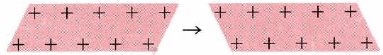
- Malleability and Ductility: The electron-sea model of metals not only explains their electrical properties but their malleability and ductility as well. The sea of electrons surrounding the protons acts like a cushion, and so when the metal is hammered on, for instance, the overall composition of the structure of the metal is not harmed or changed. The protons may be rearranged but the sea of electrons with adjust to the new formation of protons and keep the metal intact. When one layer of ions in an electron sea moves along one space with respect to the layer below it, the crystal structure does not fracture but is only deformed (Figure \(\PageIndex{3}\)).
- Heat capacity: This is explained by the ability of free electrons to move about the solid.
- Luster: The free electrons can absorb photons in the "sea," so metals are opaque-looking. Electrons on the surface can bounce back light at the same frequency that the light hits the surface, therefore the metal appears to be shiny.
However, these observations are only qualitative, and not quantitative, so they cannot be tested. The "Sea of Electrons" theory stands today only as an oversimplified model of how metallic bonding works.
In a molten metal, the metallic bond is still present, although the ordered structure has been broken down. The metallic bond is not fully broken until the metal boils. That means that boiling point is actually a better guide to the strength of the metallic bond than melting point is. On melting, the bond is loosened, not broken. The strength of a metallic bond depends on three things:
- The number of electrons that become delocalized from the metal
- The charge of the cation (metal).
- The size of the cation.
A strong metallic bond will be the result of more delocalized electrons, which causes the effective nuclear charge on electrons on the cation to increase, in effect making the size of the cation smaller. Metallic bonds are strong and require a great deal of energy to break, and therefore metals have high melting and boiling points. A metallic bonding theory must explain how so much bonding can occur with such few electrons (since metals are located on the left side of the periodic table and do not have many electrons in their valence shells). The theory must also account for all of a metal's unique chemical and physical properties.
Expanding the Range of Bonding Possible
Previously, we argued that bonding between atoms can classified as range of possible bonding between ionic bonds (fully charge transfer) and covalent bonds (fully shared electrons). When two atoms of slightly differing electronegativities come together to form a covalent bond, one atom attracts the electrons more than the other; this is called a polar covalent bond. However, simple “ionic” and “covalent” bonding are idealized concepts and most bonds exist on a two-dimensional continuum described by the van Arkel-Ketelaar Triangle (Figure \(\PageIndex{4}\)).
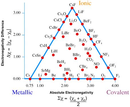
Bond triangles or van Arkel–Ketelaar triangles (named after Anton Eduard van Arkel and J. A. A. Ketelaar) are triangles used for showing different compounds in varying degrees of ionic, metallic and covalent bonding. In 1941 van Arkel recognized three extreme materials and associated bonding types. Using 36 main group elements, such as metals, metalloids and non-metals, he placed ionic, metallic and covalent bonds on the corners of an equilateral triangle, as well as suggested intermediate species. The bond triangle shows that chemical bonds are not just particular bonds of a specific type. Rather, bond types are interconnected and different compounds have varying degrees of different bonding character (for example, polar covalent bonds).
Using electronegativity - two compound average electronegativity on x-axis of Figure \(\PageIndex{4}\).
\[\sum \chi = \dfrac{\chi_A + \chi_B}{2} \label{sum}\]
and electronegativity difference on y-axis,
\[\Delta \chi = | \chi_A - \chi_B | \label{diff}\]
we can rate the dominant bond between the compounds. On the right side of Figure \(\PageIndex{4}\) (from ionic to covalent) should be compounds with varying difference in electronegativity. The compounds with equal electronegativity, such as \(\ce{Cl2}\) (chlorine) are placed in the covalent corner, while the ionic corner has compounds with large electronegativity difference, such as \(\ce{NaCl}\) (table salt). The bottom side (from metallic to covalent) contains compounds with varying degree of directionality in the bond. At one extreme is metallic bonds with delocalized bonding and at the other are covalent bonds in which the orbitals overlap in a particular direction. The left side (from ionic to metallic) is meant for delocalized bonds with varying electronegativity difference.
In general:
- Metallic bonds have low \(\Delta \chi\) and low average \(\sum\chi\).
- Ionic bonds have moderate-to-high \(\Delta \chi\) and moderate values of average \(\sum \chi\).
- Covalent bonds have moderate to high average \(\sum \chi\) and can exist with moderately low \(\Delta \chi\).
Use the tables of electronegativities (Table A2) and Figure \(\PageIndex{4}\) to estimate the following values
- difference in electronegativity (\(\Delta \chi\))
- average electronegativity in a bond (\(\sum \chi\))
- percent ionic character
- likely bond type
for the selected compounds:
- \(\ce{AsH}\) (e.g., in arsine \(AsH\))
- \(\ce{SrLi}\)
- \(\ce{KF}\).
Solution
a: \(\ce{AsH}\)
- The electronegativity of \(\ce{As}\) is 2.18
- The electronegativity of \(\ce{H}\) is 2.22
Using Equations \ref{sum} and \ref{diff}:
\[\begin{align*} \sum \chi &= \dfrac{\chi_A + \chi_B}{2} \\[4pt] &=\dfrac{2.18 + 2.22}{2} \\[4pt] &= 2.2 \end{align*}\]
\[\begin{align*} \Delta \chi &= \chi_A - \chi_B \\[4pt] &= 2.18 - 2.22 \\[4pt] &= 0.04 \end{align*}\]
- From Figure \(\PageIndex{4}\), the bond is fairly nonpolar and has a low ionic character (10% or less)
- The bonding is in the middle of a covalent bond and a metallic bond
b: \(\ce{SrLi}\)
- The electronegativity of \(\ce{Sr}\) is 0.95
- The electronegativity of \(\ce{Li}\) is 0.98
Using Equations \ref{sum} and \ref{diff}:
\[\begin{align*} \sum \chi &= \dfrac{\chi_A + \chi_B}{2} \\[4pt] &=\dfrac{0.95 + 0.98}{2} \\[4pt] &= 0.965 \end{align*}\]
\[\begin{align*} \Delta \chi &= \chi_A - \chi_B \\[4pt] &= 0.98 - 0.95 \\[4pt] &= 0.025 \end{align*}\]
- From Figure \(\PageIndex{4}\), the bond is fairly nonpolar and has a low ionic character (~3% or less)
- The bonding is likely metallic.
c: \(\ce{KF}\)
- The electronegativity of \(\ce{K}\) is 0.82
- The electronegativity of \(\ce{F}\) is 3.98
Using Equations \ref{sum} and \ref{diff}:
\[\begin{align*} \sum \chi &= \dfrac{\chi_A + \chi_B}{2} \\[4pt] &=\dfrac{0.82 + 3.98}{2} \\[4pt] &= 2.4 \end{align*}\]
\[\begin{align*} \Delta \chi &= \chi_A - \chi_B \\[4pt] &= | 0.82 - 3.98 | \\[4pt] &= 3.16 \end{align*}\]
- From Figure \(\PageIndex{4}\), the bond is fairly polar and has a high ionic character (~75%)
- The bonding is likely ionic.
Contrast the bonding of \(\ce{NaCl}\) and silicon tetrafluoride.
- Answer
-
\(\ce{NaCl}\) is an ionic crystal structure, and an electrolyte when dissolved in water; \(\Delta \chi =1.58\), average \(\sum \chi =1.79\), while silicon tetrafluoride is covalent (molecular, non-polar gas; \(\Delta \chi =2.08\), average \(\sum \chi =2.94\).
Contributors and Attributions
Jim Clark (Chemguide.co.uk)
- Daniel James Berger
- Wikipedia
Ed Vitz (Kutztown University), John W. Moore (UW-Madison), Justin Shorb (Hope College), Xavier Prat-Resina (University of Minnesota Rochester), Tim Wendorff, and Adam Hahn.