5.1: Quantum Canonical Ensemble

Last updated
Save as PDF

Page ID: 285772

\( \newcommand{\vecs}[1]{\overset { \scriptstyle \rightharpoonup} {\mathbf{#1}} } \) \( \newcommand{\vecd}[1]{\overset{-\!-\!\rightharpoonup}{\vphantom{a}\smash {#1}}} \)\(\newcommand{\id}{\mathrm{id}}\) \( \newcommand{\Span}{\mathrm{span}}\) \( \newcommand{\kernel}{\mathrm{null}\,}\) \( \newcommand{\range}{\mathrm{range}\,}\) \( \newcommand{\RealPart}{\mathrm{Re}}\) \( \newcommand{\ImaginaryPart}{\mathrm{Im}}\) \( \newcommand{\Argument}{\mathrm{Arg}}\) \( \newcommand{\norm}[1]{\| #1 \|}\) \( \newcommand{\inner}[2]{\langle #1, #2 \rangle}\) \( \newcommand{\Span}{\mathrm{span}}\) \(\newcommand{\id}{\mathrm{id}}\) \( \newcommand{\Span}{\mathrm{span}}\) \( \newcommand{\kernel}{\mathrm{null}\,}\) \( \newcommand{\range}{\mathrm{range}\,}\) \( \newcommand{\RealPart}{\mathrm{Re}}\) \( \newcommand{\ImaginaryPart}{\mathrm{Im}}\) \( \newcommand{\Argument}{\mathrm{Arg}}\) \( \newcommand{\norm}[1]{\| #1 \|}\) \( \newcommand{\inner}[2]{\langle #1, #2 \rangle}\) \( \newcommand{\Span}{\mathrm{span}}\)\(\newcommand{\AA}{\unicode[.8,0]{x212B}}\)

Density Matrix

We have occasionally referred to the quantum-mechanical density matrix \(\rho\) in previous sections. Before we discuss quantum ensembles, we need to fully specify this concept.

The microstates that can be assumed by a system in a quantum ensemble are specified by a possible set of wavefunctions \(\psi_i \ (i = 1\ldots r)\). The probability or population of the \(i^\mathrm{th}\) microstate is denoted as \(P_i\), and for the continuous case the probability density for a given wavefunction is denoted as \(p(\psi)\). The density operator is then given by

\[\begin{align} & \widehat{\rho} = \sum_{i=0}^{r-1} P_i \left|\psi_i\right\rangle \left\langle \psi_i \right| \ \mathrm{(discrete)} \\ & \widehat{\rho} = \int_\psi p(\psi) \left|\psi_i\right\rangle \left\langle \psi_i \right| \ \mathrm{(continuous)} \ . \label{eq:qm_density_operator}\end{align}\]

Note that the discrete case is closely related to the problem with \(r\) energy levels that we discussed in deriving the Boltzmann distribution for a classical canonical ensemble. The density operator can be expressed as a density matrix \(\rho\) with respect to a set of basis functions \(\left| k \right\rangle\). For exact computations the basis functions must form a countable complete set that allows for expressing the system wavefunctions \(\psi_i\) as linear combinations of basis functions. For approximate computations, it suffices that this linear combination is a good approximation. The matrix elements of the density matrix are then given by

\[\begin{align} & \rho_{nm} = \sum_{i=0}^{r-1} P_i \left\langle m \left|\psi_i\right\rangle \left\langle \psi_i \right| n \right\rangle \ \mathrm{(discrete)} \\ & \rho_{nm} = \int_\psi p(\psi) \left\langle m\left|\psi_i\right\rangle \left\langle \psi_i \right| n \right\rangle \ \mathrm{(continuous)} \ .\end{align}\]

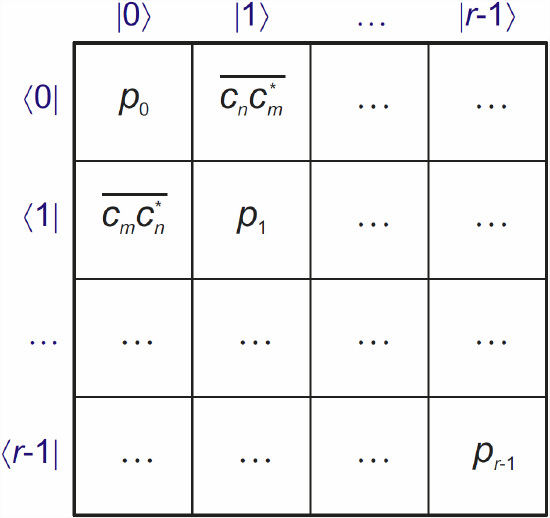
With the complex coefficients \(c_k\) in the linear combination representation \(|\psi\rangle = \sum_k c_k |k\rangle\), the matrix elements are

\[\rho_{nm} = \overline{c_n c_m^\ast} \ ,\]

where the asterisk denotes the complex conjugate and the bar for once denotes the ensemble average. It follows that diagonal elements (\(m=n\)) are necessarily real, \(\rho_{nn} = |c_n|^2\) and that \(\rho_{mn}\) is the complex conjugate of \(\rho_{nm}\). Therefore, the density matrix is Hermitian and the density operator is self-adjoint. The matrix dimension is the number of basis functions. It is often convenient to use the eigenfunctions of the system Hamiltonian \(\widehat{\mathcal{H}}\) as the basis functions, but the concept of the density matrix is not limited to this choice. The meaning of elemnts of the density matrix is visualized in Figure \(\PageIndex{1}\).

That the density matrix can be expressed in the basis of eigenstates does not imply that the ensemble can be represented as consisting of only eigenstates, as erroneously stated by Swendsen . Off-diagonal elements of the density matrix denote coherent superpositions of eigenstates, or short coherences. This is not apparent in Swendsen’s simple example where coherence is averaged to zero by construction. The ensemble can be represented as consisting of only eigenstates if coherence is absent. In that case the density matrix is diagonal in the eigenbasis. Diagonal elements of the density matrix denote populations of basis states.

Density matrix for a system with r states numbered | 0 \rangle, | 1 \rangle, …| r - 1 \rangle. The columns correspond to kets, the rows to bras of the wavefunctions corresponding to these states. Diagonal elements p_k = \rho_{kk} denote state populations and are real numbers. Off-diagonal elements \overline{c_n c_m^\ast} = \rho_{nm} are complex numbers and denote coherent superpositions of states |n \rangle and |m \rangle or, short, coherences. — Figure \(\PageIndex{1}\): Density matrix for a system with \(r\) states numbered \(| 0 \rangle\), \(| 1 \rangle\), …\(| r - 1 \rangle\). The columns correspond to kets, the rows to bras of the wavefunctions corresponding to these states. Diagonal elements \(p_k = \rho_{kk}\) denote state populations and are real numbers. Off-diagonal elements \(\overline{c_n c_m^\ast} = \rho_{nm}\) are complex numbers and denote coherent superpositions of states \(|n \rangle\) and \(|m \rangle\) or, short, coherences.

In quantum mechanics, it is well defined what information we can have about the macrostate of a system, because quantum measurements are probabilistic even for a microstate. We can observe only quantities that are quantum-mechanical observables and these observables are represented by operators \(\widehat{A}\). It can be shown that the expectation value \(\left\langle \widehat{A} \right\rangle\) of any observable can be computed from the density matrix by

\[\left\langle \widehat{A} \right\rangle = \mathrm{Trace}\left\{ \widehat{\rho} \widehat{A} \right\} \ ,\]

where we have used operator notation for \(\widehat{\rho}\) to point out that \(\widehat{\rho}\) and \(\widehat{A}\) must be expressed in the same basis.

Since the expectation values of all observables are the full information that we can have on a quantum system, the density matrix specifies the full information that we can have on the ensemble. However, the density matrix does not fully specify the ensemble itself, i.e., we cannot infer the probabilities \(P_i\) or probability density function \(\rho(\psi)\) from the density matrix (Swendsen gives a simple example ). This is another example for the information loss on microstates that comes about when we can only observe macrostates and that is conceptually equivalent to entropy. The von-Neumann entropy can be computed from the density matrix by Equation \ref{eq:von_Neumann_entropy}).

We note that there is one important distinction between classical and quantum-mechanical observations for an individual system. In the quantum case we can specify only an expectation value, and the second and third Penrose postulates (Section [Penrose_postulates]) do not apply: neither can we simultaneously measure all observables (they may be incompatible), nor is the outcome of a later measurement independent of the current measurement. However, quantum uncertainty is much smaller than measurement errors for the large ensembles that we treat by statistical thermodynamics. Hence, the Penrose postulates apply to the quantum-mechanical ensembles that represent macrostates, although they do not apply to the microstates.

If all systems in a quantum ensemble populate the same microstate, i.e., they correspond to the same wavefunction, the ensemble is said to be in a pure state. A pure state corresponds to minimum rather than maximum entropy. Otherwise the system is said to be in a mixed state.

Quantum Partition Function

Energy quantization leads to a difficulty in using the microcanonical ensemble. The difficulty arises because the microcanonical ensemble requires constant energy, which restricts our abilities to assign probabilities in a set of discrete energy levels. However, as we derived the Boltzmann distribution, partition function, entropy and all other state functions for classical systems from the canonical ensemble anyway, we can simply ignore this problem. The canonical ensemble is considered to be at thermal equilibrium with a heat bath (environment) of infinite size. It does not matter whether this heat bath is of classical or quantum mechanical nature. For an infinitely sized quantum system, the energy spectrum is continuous, which allows us to exchange energy between the bath and any constituent system of the quantum canonical ensemble at will.

We can derive Boltzmann distribution and partition function for the density matrix by analogy to the classical case. For that we consider the density matrix in the eigenbasis. The energies of the eigenstates are the eigenvalues \(\epsilon_i\) of the Hamiltonian \(\mathcal{H}\). All arguments and mathematical steps from Section [subsection:Boltzmann] still apply, with a single exception: Quantum mechanics allows for microstates that are coherent superpositions of eigenstates. The classical derivation carries over if and only if we can be sure that the equilibrium density matrix can be expressed without contributions from such microstates, which would lead to off-diagonal elements in the representation in the eigenbasis of \(\mathcal{\widehat{H}}\). This argument can indeed be made. Any superposition of two eigenstates \(|n\rangle\) and \(|m\rangle\) with amplitudes \(|c_n|\) and \(|c_m|\) can be realized with arbitrary phase difference \(\Delta \phi\) between the two eigenfunctions. The microstates with the same \(|c_n|\) and \(|c_m|\) but different \(\Delta \phi\) all have the same energy. The entropy of a subensemble that populates these microstates is maximal if the distribution of phase differences \(\Delta \phi\) is uniform in the interval \([0,2\pi)\). In that case \(\overline{c_m^\ast c_n}\) vanishes, i.e., such subensembles will not contribute off-diagonal elements to the equilibrium density matrix.

We can now arrange the \(e^{-\epsilon_i/k_\mathrm{B} T}\) in matrix form,

\[\xi = e^{-\mathcal{\widehat{H}}/k_\mathrm{B} T} \ ,\]

with the matrix elements \(\xi_{ii} = e^{-\epsilon_i/k_\mathrm{B} T}\) and \(\xi_{ij} = 0\) for \(i \neq j\). The partition function is the sum of all the diagonal elements of this matrix, i.e. the trace of \(\xi\). Hence,

\[\widehat{\rho}_\mathrm{eq} = \frac{e^{-\mathcal{\widehat{H}}/k_\mathrm{B} T}}{\mathrm{Trace}\left\{ e^{-\mathcal{\widehat{H}}/k_\mathrm{B} T} \right\}} \ , \label{eq:rho_eq} \]

where we have used operator notation. This implies that Equation \ref{eq:rho_eq} can be evaluated in any basis, not only the eigenbasis of \(\widehat{\mathcal{H}}\). In a different basis, \(e^{-\epsilon_i/k_\mathrm{B} T}\) needs to be computed as a matrix exponential and, in general, the density matrix \(\rho_\mathrm{eq}\) will have non-zero off-diagonal elements in such a different basis.

The quantum-mechanical partition function,

\[Z = \mathrm{Trace}\left\{ e^{-\mathcal{\widehat{H}}/k_\mathrm{B} T} \right\} \ , \label{eq:qm_z} \]

is independent of the choice of basis, as the trace of a matrix is invariant under unitary transformations. Note that we have used a capital \(Z\) for a molecular partition function. This is appropriate, as the trace of \(\widehat{\rho}_\mathrm{eq}\) in Equation \ref{eq:rho_eq} is unity. In the eigenbasis, the diagonal elements of \(\rho_\mathrm{eq}\) are the populations of the eigenstates at thermal equilibrium. There is no coherence for a sufficiently large quantum ensemble at thermal equilibrium.

We note that the density matrix at thermal equilibrium can be derived in a more strict manner by explicitly considering a system that includes both the canonical ensemble and the heat bath and by either tracing out the degrees of freedom of the heat bath or relying on a series expansion that reduces to only two terms in the limit of an infinite heat bath .

When approaching zero absolute temperature, the matrix element of \(\rho\) in the eigenbasis that corresponds to the lowest energy \(\epsilon_i\) becomes much larger than all the others. At \(T=0\), the corresponding ground state is exclusively populated and the ensemble is in a pure state if there is just one state with this energy. For \(T \rightarrow \infty\) on the other hand, differences between the diagonal matrix elements vanish and all states are equally populated. The ensemble is in a maximally mixed state.