
8.68: A Simple Solution to Deutsch's Problem
- Page ID
- 148506

\( \newcommand{\vecs}[1]{\overset { \scriptstyle \rightharpoonup} {\mathbf{#1}} } \)
\( \newcommand{\vecd}[1]{\overset{-\!-\!\rightharpoonup}{\vphantom{a}\smash {#1}}} \)
\( \newcommand{\id}{\mathrm{id}}\) \( \newcommand{\Span}{\mathrm{span}}\)
( \newcommand{\kernel}{\mathrm{null}\,}\) \( \newcommand{\range}{\mathrm{range}\,}\)
\( \newcommand{\RealPart}{\mathrm{Re}}\) \( \newcommand{\ImaginaryPart}{\mathrm{Im}}\)
\( \newcommand{\Argument}{\mathrm{Arg}}\) \( \newcommand{\norm}[1]{\| #1 \|}\)
\( \newcommand{\inner}[2]{\langle #1, #2 \rangle}\)
\( \newcommand{\Span}{\mathrm{span}}\)
\( \newcommand{\id}{\mathrm{id}}\)
\( \newcommand{\Span}{\mathrm{span}}\)
\( \newcommand{\kernel}{\mathrm{null}\,}\)
\( \newcommand{\range}{\mathrm{range}\,}\)
\( \newcommand{\RealPart}{\mathrm{Re}}\)
\( \newcommand{\ImaginaryPart}{\mathrm{Im}}\)
\( \newcommand{\Argument}{\mathrm{Arg}}\)
\( \newcommand{\norm}[1]{\| #1 \|}\)
\( \newcommand{\inner}[2]{\langle #1, #2 \rangle}\)
\( \newcommand{\Span}{\mathrm{span}}\) \( \newcommand{\AA}{\unicode[.8,0]{x212B}}\)
\( \newcommand{\vectorA}[1]{\vec{#1}} % arrow\)
\( \newcommand{\vectorAt}[1]{\vec{\text{#1}}} % arrow\)
\( \newcommand{\vectorB}[1]{\overset { \scriptstyle \rightharpoonup} {\mathbf{#1}} } \)
\( \newcommand{\vectorC}[1]{\textbf{#1}} \)
\( \newcommand{\vectorD}[1]{\overrightarrow{#1}} \)
\( \newcommand{\vectorDt}[1]{\overrightarrow{\text{#1}}} \)
\( \newcommand{\vectE}[1]{\overset{-\!-\!\rightharpoonup}{\vphantom{a}\smash{\mathbf {#1}}}} \)
\( \newcommand{\vecs}[1]{\overset { \scriptstyle \rightharpoonup} {\mathbf{#1}} } \)
\( \newcommand{\vecd}[1]{\overset{-\!-\!\rightharpoonup}{\vphantom{a}\smash {#1}}} \)
\(\newcommand{\avec}{\mathbf a}\) \(\newcommand{\bvec}{\mathbf b}\) \(\newcommand{\cvec}{\mathbf c}\) \(\newcommand{\dvec}{\mathbf d}\) \(\newcommand{\dtil}{\widetilde{\mathbf d}}\) \(\newcommand{\evec}{\mathbf e}\) \(\newcommand{\fvec}{\mathbf f}\) \(\newcommand{\nvec}{\mathbf n}\) \(\newcommand{\pvec}{\mathbf p}\) \(\newcommand{\qvec}{\mathbf q}\) \(\newcommand{\svec}{\mathbf s}\) \(\newcommand{\tvec}{\mathbf t}\) \(\newcommand{\uvec}{\mathbf u}\) \(\newcommand{\vvec}{\mathbf v}\) \(\newcommand{\wvec}{\mathbf w}\) \(\newcommand{\xvec}{\mathbf x}\) \(\newcommand{\yvec}{\mathbf y}\) \(\newcommand{\zvec}{\mathbf z}\) \(\newcommand{\rvec}{\mathbf r}\) \(\newcommand{\mvec}{\mathbf m}\) \(\newcommand{\zerovec}{\mathbf 0}\) \(\newcommand{\onevec}{\mathbf 1}\) \(\newcommand{\real}{\mathbb R}\) \(\newcommand{\twovec}[2]{\left[\begin{array}{r}#1 \\ #2 \end{array}\right]}\) \(\newcommand{\ctwovec}[2]{\left[\begin{array}{c}#1 \\ #2 \end{array}\right]}\) \(\newcommand{\threevec}[3]{\left[\begin{array}{r}#1 \\ #2 \\ #3 \end{array}\right]}\) \(\newcommand{\cthreevec}[3]{\left[\begin{array}{c}#1 \\ #2 \\ #3 \end{array}\right]}\) \(\newcommand{\fourvec}[4]{\left[\begin{array}{r}#1 \\ #2 \\ #3 \\ #4 \end{array}\right]}\) \(\newcommand{\cfourvec}[4]{\left[\begin{array}{c}#1 \\ #2 \\ #3 \\ #4 \end{array}\right]}\) \(\newcommand{\fivevec}[5]{\left[\begin{array}{r}#1 \\ #2 \\ #3 \\ #4 \\ #5 \\ \end{array}\right]}\) \(\newcommand{\cfivevec}[5]{\left[\begin{array}{c}#1 \\ #2 \\ #3 \\ #4 \\ #5 \\ \end{array}\right]}\) \(\newcommand{\mattwo}[4]{\left[\begin{array}{rr}#1 \amp #2 \\ #3 \amp #4 \\ \end{array}\right]}\) \(\newcommand{\laspan}[1]{\text{Span}\{#1\}}\) \(\newcommand{\bcal}{\cal B}\) \(\newcommand{\ccal}{\cal C}\) \(\newcommand{\scal}{\cal S}\) \(\newcommand{\wcal}{\cal W}\) \(\newcommand{\ecal}{\cal E}\) \(\newcommand{\coords}[2]{\left\{#1\right\}_{#2}}\) \(\newcommand{\gray}[1]{\color{gray}{#1}}\) \(\newcommand{\lgray}[1]{\color{lightgray}{#1}}\) \(\newcommand{\rank}{\operatorname{rank}}\) \(\newcommand{\row}{\text{Row}}\) \(\newcommand{\col}{\text{Col}}\) \(\renewcommand{\row}{\text{Row}}\) \(\newcommand{\nul}{\text{Nul}}\) \(\newcommand{\var}{\text{Var}}\) \(\newcommand{\corr}{\text{corr}}\) \(\newcommand{\len}[1]{\left|#1\right|}\) \(\newcommand{\bbar}{\overline{\bvec}}\) \(\newcommand{\bhat}{\widehat{\bvec}}\) \(\newcommand{\bperp}{\bvec^\perp}\) \(\newcommand{\xhat}{\widehat{\xvec}}\) \(\newcommand{\vhat}{\widehat{\vvec}}\) \(\newcommand{\uhat}{\widehat{\uvec}}\) \(\newcommand{\what}{\widehat{\wvec}}\) \(\newcommand{\Sighat}{\widehat{\Sigma}}\) \(\newcommand{\lt}{<}\) \(\newcommand{\gt}{>}\) \(\newcommand{\amp}{&}\) \(\definecolor{fillinmathshade}{gray}{0.9}\)This tutorial is closely related to the preceding one. A certain function of x maps {0,1} to {0,1}. The four possible outcomes of the evaluation of f(x) are given in tabular form.
\[ \begin{pmatrix} \text{x} & ' & 0 & 1 & ' & 0 & 1 & ' & 0 & 1 & ' & 0 & 1 \\ \text{f(x)} & ' & 0 & 0 & ' & 1 & 1 & ' & 0 & 1 & ' & 1 & 0 \end{pmatrix} \nonumber \]
In the previous tutorial we established that the circuit shown below yields the result given in the right most section of the table. In other words, f(x) is a balanced function, because \(f(0) \neq f(1)\), as is the result immediately to its left. The results in the first two sections are labelled constant because \( f(0) = f(1)\).

where, for example
\[ \begin{matrix} |0 \rangle = \begin{pmatrix} 1 \\ 0 \end{pmatrix} & |1 \rangle = \begin{pmatrix} 0 \\ 1 \end{pmatrix} \end{matrix} \nonumber \]
This circuit carries out,
\[ \hat{U}_f |x \rangle |0 \rangle = |x \rangle | f(x) \rangle \nonumber \]
where Uf (controlled-NOT, followed by a NOT operation on the lower wire) is a unitary operator that accepts input |x> on the top wire and places f(x) on the bottom wire.
From the classical perspective, if the question (as asked by Deutsch) is whether f(x) is constant or balanced then one must calculate both f(0) and f(1) to answer the question. Deutsch pointed out that quantum superpositions and the interference effects between them allow the answer to be given with one pass through a modified version of the circuit as shown here.
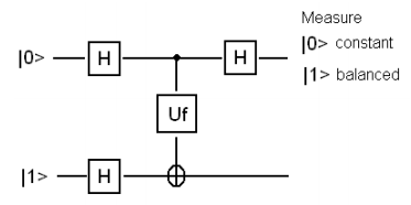
The input |0>|1> is followed by a Hadamard gate on each wire. As is well known the Hadamard operation creates the following superposition states.
\[ \begin{matrix} \text{H} \begin{pmatrix} 1 \\ 0 \end{pmatrix} = \frac{1}{ \sqrt{2}} \begin{pmatrix} 1 \\ 1 \end{pmatrix} & \text{H} \begin{pmatrix} 0 \\ 1 \end{pmatrix} = \frac{1}{ \sqrt{2}} \begin{pmatrix} 1 \\ -1 \end{pmatrix} \end{matrix} \nonumber \]
Therefore the Hadamard operations transform the input state to the following two-qubit state which is fed to Uf.
\[ |x \rangle |y \rangle = \frac{1}{ \sqrt{2}} \begin{pmatrix} 1 \\ 1 \end{pmatrix} \otimes \frac{1}{ \sqrt{2}} \begin{pmatrix} 1 \\ -1 \end{pmatrix} = \frac{1}{2} \begin{pmatrix} 1 \\ -1 \\ 1 \\ -1 \end{pmatrix} \nonumber \]
Uf processes its input to generate the following output.
\[ \hat{U}_f |x \rangle |y \rangle = |x \rangle | \text{mod}_2 (y + f(x)) \rangle = |x \rangle |y \oplus f(x) \rangle \nonumber \]
To facilitate an algebraic analysis of the circuit operation the input state is written as,
\[ |x \rangle |y \rangle = \frac{1}{ \sqrt{2}} \left[ |0 \rangle +|1 \rangle \right] \frac{1}{ \sqrt{2}} \left[ |0 \rangle - |1 \rangle \right] = \frac{1}{2} \left[ |0 \rangle |0 \rangle - |0 \rangle |1 \rangle + |1 \rangle |0 \rangle - |1 \rangle |1 \rangle \right] \nonumber \]
In this format Uf creates the following output state.
\[ \Psi_{out} = \frac{1}{2} \left[ |0 \rangle | f(0) \rangle - |0 \rangle |1 \oplus f(0) \rangle + |1 \rangle | f(1) \rangle - |1 \rangle |1 \oplus f(1) \rangle \right] \nonumber \]
As the table shows there are four possible outcomes depending on whether the function is constant (the first two) or balanced (the second two).
\[ \begin{matrix} \Psi_{out} \xrightarrow[f(0) = 0]{f(0) = f(1)} \frac{1}{2} \left[ |0 \rangle |0 \rangle - |0 \rangle |1 \rangle + |1 \rangle |0 \rangle - |1 \rangle |1 \rangle \right] = \frac{1}{2} \left( |0 \rangle + |1 \rangle \right) \left( |0 \rangle - |1 \rangle \right) \\ \Psi_{out} \xrightarrow[f(0) = 1]{f(0) = f(1)} \frac{1}{2} \left[ |0 \rangle |1 \rangle - |0 \rangle |0 \rangle + |1 \rangle |1 \rangle - |1 \rangle |0 \rangle \right] = - \frac{1}{2} \left( |0 \rangle + |1 \rangle \right) \left( |0 \rangle - |1 \rangle \right) \\ \Psi_{out} \xrightarrow[f(0) = 0]{f(0) \neq f(1)} \frac{1}{2} \left[ |0 \rangle |0 \rangle - |0 \rangle |1 \rangle + |1 \rangle |1 \rangle - |1 \rangle |0 \rangle \right] = \frac{1}{2} \left( |0 \rangle + |1 \rangle \right) \left( |0 \rangle - |1 \rangle \right) \\ \Psi_{out} \xrightarrow[f(0) = 1]{f(0) \neq f(1)} \frac{1}{2} \left[ |0 \rangle |1 \rangle - |0 \rangle |0 \rangle + |1 \rangle |0 \rangle - |1 \rangle |1 \rangle \right] = - \frac{1}{2} \left( |0 \rangle - |1 \rangle \right) \left( |0 \rangle - |1 \rangle \right) \end{matrix} \nonumber \]
The Hadamard operation (see matrix below) on the first qubit brings about the following transformations.
\[ \begin{matrix} H \frac{1}{2} \left( |0 \rangle + |1 \rangle \right) = \frac{1}{ \sqrt{2}} |0 \rangle & H \frac{1}{2} \left( |0 \rangle - |1 \rangle \right) = \frac{1}{ \sqrt{2}} |1 \rangle \end{matrix} \nonumber \]
The four possible output states are now,
\[ \begin{matrix} \Psi_{out} \xrightarrow[f(0) = 0]{f(0) = f(1)} \frac{1}{ \sqrt{2}} |0 \rangle \left( |0 \rangle - |1 \rangle \right) = \frac{1}{ \sqrt{2}} \begin{pmatrix} 1 \\ -1 \\ 0 \\ 0 \end{pmatrix} & \Psi_{out} \xrightarrow[f(0) = 1]{f(0) = f(1)} - \frac{1}{ \sqrt{2}} |0 \rangle \left( |0 \rangle - |1 \rangle \right) = \frac{1}{ \sqrt{2}} \begin{pmatrix} -1 \\ 1 \\ 0 \\ 0 \end{pmatrix} \\ \Psi_{out} \xrightarrow[f(0) = 0]{f(0) \neq f(1)} \frac{1}{ \sqrt{2}} |1 \rangle \left( |0 \rangle - |1 \rangle \right) = \frac{1}{ \sqrt{2}} \begin{pmatrix} 0 \\ 0 \\ 1 \\ -1 \end{pmatrix} & \Psi_{out} \xrightarrow[f(0) = 1]{f(0) \neq f(1)} - \frac{1}{ \sqrt{2}} |1 \rangle \left( |0 \rangle - |1 \rangle \right) = \frac{1}{ \sqrt{2}} \begin{pmatrix} 0 \\ 0 \\ -1 \\ 1 \end{pmatrix} \end{matrix} \nonumber \]
Quantum mechanics answers Deutsch's question with a single measurement. A measurement on the first qubit reveals whether the function is constant (|0>) or balanced (|1>).
We now look at the same calculation using matrix algebra. The required quantum operators in matrix form are:
\[ \begin{matrix} \text{I} = \begin{pmatrix} 1 & 0 \\ 0 & 1 \end{pmatrix} & \text{NOT} = \begin{pmatrix} 0 & 1 \\ 1 & 0 \end{pmatrix} & \text{H} = \frac{1}{ \sqrt{2}} \begin{pmatrix} 1 & 1 \\ 1 & -1 \end{pmatrix} & \text{CNOT} = \begin{pmatrix} 1 & 0 & 0 & 0 \\ 0 & 1 & 0 & 0 \\ 0 & 0 & 0 & 1 \\ 0 & 0 & 1 & 0 \end{pmatrix} \end{matrix} \nonumber \]
Kronecker is Mathcad's command for carrying out matrix tensor multiplication. Note that the identity operator is required when a wire is not involved in an operation.
\[ \begin{matrix} \text{U}_f = \text{kronecker(I, NOT) CNOT} & \text{QuantumCircuit} = \text{kronecker(H, I) U}_f ~ \text{kronecker(H, H)} \end{matrix} \nonumber \]
Input state:
\[ \begin{matrix} |0 \rangle |1 \rangle = \begin{pmatrix} 1 \\ 0 \end{pmatrix} \otimes \begin{pmatrix} 0 \\ 1 \end{pmatrix} = \begin{pmatrix} 0 \\ 1 \\ 0 \\ 0 \end{pmatrix} & \text{QuantumCircuit} \begin{pmatrix} 0 \\ 1 \\ 0 \\ 0 \end{pmatrix} = \begin{pmatrix} 0 \\ 0 \\ -0.707 \\ 0.707 \end{pmatrix} \end{matrix} \nonumber \]
Comparing this with the previous algebraic analysis, we see that the quantum circuit produces the result \( f(0) \neq f(1)\) with f(0) = 1, which we already knew from previous work.
The measurement on the first qubit is implemented with projection operators |0><1|, and confirms that the function is not constant but belongs to the balanced category.
\[ \begin{matrix} \text{kronecker} \left[ \begin{pmatrix} 1 \\ 0 \end{pmatrix} \begin{pmatrix} 1 \\ 0 \end{pmatrix}^T, ~ \text{I} \right] \text{QuantumCircuit} \begin{pmatrix} 0 \\ . \\ 0 \\ 0 \end{pmatrix} = \begin{pmatrix} 0 \\ 0 \\ 0 \\ 0 \end{pmatrix} & \text{Top qubit is not |0 >.} \\ \text{kronecker} \left[ \begin{pmatrix} 0 \\ 1 \end{pmatrix} \begin{pmatrix} 0 \\ 1 \end{pmatrix}^T,~\text{I} \right] \text{QuantumCircuit} \begin{pmatrix} 0 \\ 1 \\ 0 \\ 0 \end{pmatrix} = \begin{pmatrix} 0 \\ 0 \\ -0.707 \\ 0.707 \end{pmatrix} & \text{Top qubit is |1 >.} \end{matrix} \nonumber \]
This could have also been easily determined by inspection:
\[ \frac{1}{ \sqrt{2}} \begin{pmatrix} 0 \\ 0 \\ -1 \\ 1 \end{pmatrix} = \begin{pmatrix} 0 \\ 1 \end{pmatrix} \frac{1}{ \sqrt{2}} \left[ \begin{pmatrix} 0 \\ 1 \end{pmatrix} - \begin{pmatrix} 1 \\ 0 \end{pmatrix} \right] \nonumber \]
The following provides an algebraic analysis of the Deutsch algorithm.
\[ \begin{matrix} |0 \rangle & \triangleright & \fbox{H} & \cdots & \cdot & \cdots & \fbox{H} & \triangleright & \text{measure} \frac{ |0 \rangle \text{ constant}}{|1 \rangle \text{ balance}} \\ ~ & ~ & ~ & ~ | \\ |1 \rangle & \triangleright & \fbox{H} & \cdots & \oplus & \fbox{NOT} & \cdots \end{matrix} \nonumber \]
Hadamard operation:
\[ \begin{matrix} \text{H} |0 \rangle \rightarrow \frac{1}{ \sqrt{2}} \left[ |0 \rangle + |1 \rangle \right] & \text{H} |1 \rangle \rightarrow \frac{1}{ \sqrt{2}} \left[ |0 \rangle - |1 \rangle \right] \end{matrix} \nonumber \]
\[ \begin{matrix} \text{NOT} & \begin{pmatrix} \text{0 to 1} \\ \text{1 to 0} \end{pmatrix} & \text{CNOT} & \begin{pmatrix} \text{Decimal} & \text{Binary} & \text{to} & \text{Binary} & \text{Decimal} \\ 0 & 00 & \text{to} & 00 & 0 \\ 1 & 01 & \text{to} & 01 & 1 \\ 2 & 10 & \text{to} & 11 & 3 \\ 3 & 11 & \text{to} & 10 & 2 \end{pmatrix} \end{matrix} \nonumber \]
\[ \begin{matrix} |01 \rangle \\ \text{H} \otimes \text{H} \\ \frac{1}{ \sqrt{2}} \left[ |0 \rangle + |1 \rangle \right] \frac{1}{ \sqrt{2}} \left[ |0 \rangle - |1 \rangle \right] = \frac{1}{2} \left[ |00 \rangle - |01 \rangle + |10 \rangle - |11 \rangle \right] \\ \text{CNOT} \\ \frac{1}{2} \left[ |00 \rangle - |01 \rangle + 11 \rangle - |10 \rangle \right] = \frac{1}{2} \left( |0 \rangle - |1 \rangle \right) \left( |0 \rangle - |1 \rangle \right) \\ \text{I} \otimes \text{NOT} \\ \frac{1}{2} \left[ \left( |0 \rangle - |1 \rangle \right) \left( |1 \rangle - |1 \rangle \right) \right] \\ \text{H} \otimes \text{I} \\ |1 \rangle \frac{1}{ \sqrt{2}} \left( |1 \rangle - |0 \rangle \right) \end{matrix} \nonumber \]
The top wire contains |1 > indicating the function is balanced.
The Hadamard operation is actually a simple example of a Fourier transform. In other words, the final step of Deutsch's algorithm is to carry out a Fourier transform on the input wire. This also occurs on the input wires in Grover's search algorithm, Simon's query algorithm and Shor's factorization algorithm.