8.38: Mermin's Version of Bohm's EPR Gedanken Experiment Using Tensor Algebra

The purpose of this tutorial is to summarize a gedanken experiment that reveals a conflict between the predictions of local realism and quantum mechanics. The thought experiment was presented by N. David Mermin in the American Journal of Physics (October 1981, pp 941-943) and Physics Today (April 1985, pp 38-47). In this summary the quantum mechanical analysis employs tensor algebra.

A spin-1/2 pair is prepared in a singlet state and the individual particles travel in opposite directions to a pair of detectors which are set up to measure spin in three directions in x-z plane: along the z-axis, and angles of 120 and 240 degrees with respect to the z-axis. The detector settings are labeled 1, 2 and 3, respectively.

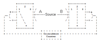
The switches on the detectors are set randomly so that all nine possible settings of the two detectors occur with equal frequency.

Local realism holds that objects have properties independent of measurement and that measurements at one location on a particle cannot influence measurements of another particle at another distant location even if the particles were created in the same event. Local realism maintains that the spin-1/2 particles carry instruction sets which dictate the results of subsequent measurements. That is, prior to measurement the particles are in a well-defined state.

The following table presents the experimental results expected on the basis of local realism. Singlet spin states have opposite spin values for each of the three measurement directions. For example, if A's spin state is (+-+), then B's spin state is (-+-). If A's detector is set to spin direction "1" and B's detector is set to spin direction "3" the measured result will be recorded as +-.

Note that there are eight spin states and nine possible detector settings, giving 72 possible measurement outcomes all of which are equally probable.

The table shows that the assumption that the singlet-state particles have well-defined spin states prior to measurement requires that the probability the detectors will register opposite spin values is 0.67 (48/72). If the detectors are set to the same direction, they always register different spin values (24/24), and if they are set to different directions the probability they will register different spin values is 0.50 (24/48).

Now we show that a quantum mechanical analysis is in sharp disagreement with the local realistic view just presented.

The natural base states for this quantum analysis are spin-up and spin-down in the z-direction.

\[ \begin{matrix} S_{zu} = \begin{pmatrix} 1 \\ 0 \end{pmatrix} & S_{zd} = \begin{pmatrix} 0 \\ 1 \end{pmatrix} \end{matrix} \nonumber \]

The singlet state produced by the source (fermions have anti-symmetric wave functions and are indistinguishable) in tensor format is,

\[ \begin{matrix} | \Psi \rangle = \frac{1}{ \sqrt{2}} \left[ | \uparrow \rangle_1 | \downarrow \rangle_2 - | \downarrow \rangle_1 | \uparrow \rangle_2 \right] = \frac{1}{ \sqrt{2}} \left[ \begin{pmatrix} 1 \\ 0 \end{pmatrix} \otimes \begin{pmatrix} 0 \\ 1 \end{pmatrix} - \begin{pmatrix} 0 \\ 1 \end{pmatrix} \otimes \begin{pmatrix} 1 \\ 0 \end{pmatrix} \right] = \frac{1}{ \sqrt{2}} \begin{pmatrix} 0 \\ 1 \\ -1 \\ 0 \end{pmatrix} & \Psi = \frac{1}{ \sqrt{2}} \begin{pmatrix} 0 \\ 1 \\ -1 \\ 0 \end{pmatrix} \end{matrix} \nonumber \]

The single particle spin operator in the x-z plane is constructed from the Pauli spin operators in the xand z-directions. ϕ is the angle of orientation of the measurement magnet with the z-axis. Note that the Pauli operators measure spin in units of h/4π. This provides for some mathematical clarity in the forthcoming analysis.

\[ \begin{matrix} \sigma_z = \begin{pmatrix} 1 & 0 \\ 0 & -1 \end{pmatrix} & \sigma_x = \begin{pmatrix} 0 & 1 \\ 1 & 0 \end{pmatrix} & S( \varphi) = \cos (\varphi) \sigma_z + \sin (\varphi) \sigma_x \rightarrow \begin{pmatrix} \cos (\varphi) & \sin (\varphi) \\ \sin (\varphi) & - \cos (\varphi) \end{pmatrix} \end{matrix} \nonumber \]

Obviously if ϕ or π/2 we recover σ_z and σ_x.

\[ \begin{matrix} S(0) = \begin{pmatrix} 1 & 0 \\ 0 & -1 \end{pmatrix} & S \left( \frac{ \pi}{2} \right) = \begin{pmatrix} 0 & 1 \\ 1 & 0 \end{pmatrix} \end{matrix} \nonumber \]

The spin operator for the two-particle system in tensor format is,

\[ \begin{pmatrix} \cos \varphi_A & \sin \varphi_A \\ \sin \varphi_A & - \cos \varphi_A \end{pmatrix} \otimes \begin{pmatrix} \cos \varphi_B & \sin \varphi_B \\ \sin \varphi_B & - \cos \varphi_B \end{pmatrix} = \begin{pmatrix} \cos \varphi_A \begin{pmatrix} \cos \varphi_B & \sin \varphi_B \\ \sin \varphi_B & - \cos \varphi_B \end{pmatrix} & \sin \varphi_A \begin{pmatrix} \cos \varphi_B & \sin \varphi_B \\ \sin \varphi_B & - \cos \varphi_B \end{pmatrix} \\ \sin \varphi_A \begin{pmatrix} \cos \varphi_B & \sin \varphi_B \\ \sin \varphi_B & - \cos \varphi_B \end{pmatrix} & - \cos \varphi_A \begin{pmatrix} \cos \varphi_B & \sin \varphi_B \\ \sin \varphi_B & - \cos \varphi_B \end{pmatrix} \end{pmatrix} \nonumber \]

In Mathcad the two-spin operator is written as,

\[ \text{kronecker}(S( \varphi_A),~S( \varphi_B)) \nonumber \]

In the z-basis the eigenvalues for spin-up and spin-down are +1 and -1 respectively.

\[ \begin{matrix} S_{zu}^T \sigma_z S_{zu} \rightarrow 1 & S_{zd}^T \sigma_z S_{zd} \rightarrow -1 \end{matrix} \nonumber \]

The combined measurement of both spins when the detectors have the same x-z orientation yields an expectation value of -1, because Ψ is a singlet state and the individual spins have opposite orientations.

\[ \begin{matrix} \Psi^T \text{kronecker(S, (0 deg), S(0 deg)} \Psi = -1 & \Psi^T \text{kronecker(S, (120 deg), S(120 deg)} \Psi = -1 & \Psi^T \text{kronecker(S, (240 deg), S(240 deg)} \Psi = -1 \end{matrix} \nonumber \]

These results are in agreement with the local realist predictions in the right third of the table above. When the detectors are oriented at the same angle in the x-z plane they always register opposite spin values for their respective particles. At this point, quantum mechanics appears to support the realistic position.

However, overall (considering all nine detector settings) quantum mechanics predicts that opposite spins are recorded only 50% of the time, as opposed to 67% predicted by local realism. In other words, the overall expectation value for the joint spin measurements is 0. Quantum mechanics strongly disagrees with local realism in the experiments in which the detector settings differ. In these cases, quantum theory predicts the detectors register opposite spin values 25% of the time and the same value 75% of the time: 0.25(-1) + 0.75(+1) = 0.5 as shown by the off-diagonal vlaues in the results matrix below.

\[ \begin{matrix} i = 0.2 & j = 0.2 & R_{i,~j} = \Psi^T \text{kronecker[S[i (120 deg)], (120 deg)]]} \Psi & R = \begin{pmatrix} -1 & 0.5 & 0.5 \\ 0.5 & -1& 0.5 \\ 0.5 & 0.5 & -1 \end{pmatrix} \end{matrix} \nonumber \]

Calculation of the overall spin value:

\[ \sum_i \sum_j \left[ \Psi^T \text{kronecker[S [i (120 deg)], S[j (120 deg)]]} \Psi \right] = 0 \nonumber \]

By comparison the spin expectation value based on local realism as represented by the table above is:

\[ \frac{48}{72} (-1) + \frac{24}{72}(1) = -0.333 \nonumber \]

The fact that local realism and quantum mechanics can lead to different predictions that might be adjudicated by experimental measurement was first pointed out by John S. Bell [Physics 1, 195 (1964)].

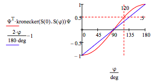
Sections 6.2, 6.3 and 11.3 of A. I. M. Rae's Quantum Mechanics, 3rd Ed. contain,in a clear and succinct fashion, the necessary mathematical background for this thought experiment. The key quantum spin correlation function of Rae's analysis (Fig 11.3) is calculated as follows in tensor format. The linear function in blue is the hidden-variable correlation function.

One more comment can be made about local realism and quantum mechanics in this particular example. If we look at the results for the first spin in the table above, its over-all expectation value is 0. There are as many +s as -s. Quantum mechanics agrees with local realism with this result in addition to the case in which the detectors have the same setting.

We can calculate the expectation values for the first spin independent of the second spin by replacing the spin operator of the second spin with the identity operator.

\[I = \begin{pmatrix} 1 & 0 \\ 0 & 1 \end{pmatrix} \nonumber \]

We see that the expectation values for the three detector orientations of the first spin are 0. In other words, the measurement results on the first spin are perfectly random.

\[ \begin{matrix} \Psi^T \text{kronecker(S, (0 deg), I} \Psi = 0 & \Psi^T \text{kronecker(S, (120 deg), I} \Psi = 0 & \Psi^T \text{kronecker(S, (240 deg), I} \Psi = 0 \end{matrix} \nonumber \]

The same holds for the second spin.

\[ \begin{matrix} \Psi^T \text{kronecker(I, S(0 deg)} \Psi = 0 & \Psi^T \text{kronecker(I, S(120 deg)} \Psi = 0 & \Psi^T \text{kronecker(I, S(240 deg)} \Psi = 0 \end{matrix} \nonumber \]

And yet when the angles are the same the measurement results (as shown above) are correlated.

\[ \begin{matrix} \Psi^T \text{kronecker(S, (0 deg), S(0 deg)} \Psi = -1 & \Psi^T \text{kronecker(S, (120 deg), S(120 deg)} \Psi = -1 & \Psi^T \text{kronecker(S, (240 deg), S(240 deg)} \Psi = -1 \end{matrix} \nonumber \]

"How is it possible that two events, each one objectively random, are always perfectly correlated." Anton Zeilinger, Nature, 8 December 2005.

All the calculations carried out above can also be done having the trace function operate on the product of the density matrix for Ψ and the matrices representing the measurement operators. Several examples are provided below.

Form the density matrix for Ψ.

\[ \rho \Psi = \Psi \Psi^T \nonumber \]

\[ \begin{matrix} tr \left( \rho \Psi \text{kronecker(S (120 deg), S(120 deg))} \right) = -1 & tr \left( \rho \Psi \text{kronecker(S (0 deg), S(120 deg))} \right) = 0.5 \end{matrix} \nonumber \]

\[ tr \left[ \sum_i \sum_j \left[ \rho \Psi \text{kronecker[S [i (120 deg)], S[j (120 deg)]} \right] \right] = 0 \nonumber \]