8.37: Another Look at Mermin's EPR Gedanken Experiment

Quantum theory is both stupendously successful as an account of the small-scale structure of the world and it is also the subject of an unresolved debate and dispute about its interpretation. J. C. Polkinghorne, The Quantum World, p. 1.

In Bohm's EPR thought experiment (Quantum Theory, 1951, pp. 611-623), both local realism and quantum mechanics were shown to be consistent with the experimental data. However, the local realistic explanation used composite spin states that were invalid according to quantum theory. The local realists countered that this was an indication that quantum mechanics was incomplete because it couldn't assign well-defined values to all observable properties prior to or independent of observation. In the 1980s N. David Mermin presented a related thought experiment [American Journal of Physics (October 1981, pp 941-943) and Physics Today (April 1985, pp 38-47)] in which the predictions of local realism and quantum mechanics disagree. As such Mermin's thought experiment represents a specific illustration of Bell's theorem.

A spin-1/2 pair is prepared in a singlet state and the individual particles travel in opposite directions to detectors which are set up to measure spin in three directions in x-z plane: along the z-axis, and angles of 120 and 240 degrees with respect to the z-axis. The detector settings are labeled 1, 2 and 3, respectively.

The switches on the detectors are set randomly so that all nine possible settings of the two detectors occur with equal frequency.

Local realism holds that objects have properties independent of measurement and that measurements at one location on a particle cannot influence measurements of another particle at a distant location even if the particles were created in the same event. Local realism maintains that the spin-1/2 particles carry instruction sets (hidden variables) which dictate the results of subsequent measurements. Prior to measurement the particles are in an unknown but well-defined state.

The following table presents the experimental results expected on the basis of local realism. Singlet spin states have opposite spin values for each of the three measurement directions. If A's spin state is (+-+), then B's spin state is (-+-). A '+' indicates spin-up and a measurement eigenvalue of +1. A '-' indicates spin-down and a measurement eigenvalue of -1. If A's detector is set to spin direction "1" and B's detector is set to spin direction "3" the measured result will be recorded as +-,with an eigenvalue of -1.

There are eight spin states and nine possible detector settings, giving 72 possible measurement outcomes all of which are equally probable. The next to bottom line of the table shows the average (expectation) value for the nine possible detector settings given the local realist spin states. When the detector settings are the same there is perfect anti-correlation between the detectors at A and B. When the detectors are set at different spin directions there is no correlation.

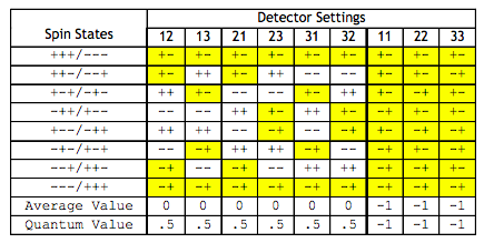
As will now be shown quantum mechanics (bottom line of the table) disagrees with this local realistic analysis. The singlet state produced by the source is the following entangled superposition, where the arrows indicate the spin orientation for any direction in the x-z plane. As noted above the directions used are 0, 120 and 240 degrees, relative to the z-axis.

\[ \begin{matrix} | \Psi \rangle = \frac{1}{ \sqrt{2}} \left[ | \uparrow \rangle_1 | \downarrow \rangle_2 - | \uparrow \rangle_1 | \downarrow \rangle_2 \right] = \frac{1}{ \sqrt{2}} \left[ \begin{pmatrix} \cos \left( \frac{ \varphi}{2} \right) \\ \sin \left( \frac{ \varphi}{2} \right) \end{pmatrix} \otimes \begin{pmatrix} - \sin \left( \frac{ \varphi}{2} \right) \\ \cos \left( \frac{ \varphi}{2} \right) \end{pmatrix} - \begin{pmatrix} - \sin \left( \frac{ \varphi}{2} \right) \\ \cos \left( \frac{ \varphi}{2} \right) \end{pmatrix} \otimes \begin{pmatrix} \cos \left( \frac{ \varphi}{2} \right) \\ \sin \left( \frac{ \varphi}{2} \right) \end{pmatrix} \right] = \frac{1}{ \sqrt{2}} \begin{pmatrix} 0 \\ 1 \\ -1 \\ 0 \end{pmatrix} & \Psi = \frac{1}{ \sqrt{2}} \begin{pmatrix} 0 \\ 1 \\ -1 \\ 0 \end{pmatrix} \end{matrix} \nonumber \]

The single particle spin operator in the x-z plane is constructed from the Pauli spin operators in the x and z-directions. ϕ is the angle of orientation of the measurement magnet with the z-axis. Note that the Pauli operators measure spin in units of h/4π. This provides for some mathematical clarity in the forthcoming analysis.

\[ \begin{matrix} \sigma_z = \begin{pmatrix} 1 & 0 \\ 0 & -1 \end{pmatrix} & \sigma_x = \begin{pmatrix} 0 & 1 \\ 1 & 0 \end{pmatrix} & S( \varphi) = \cos (\varphi) \sigma_z + \sin (\varphi) \sigma_x \rightarrow \begin{pmatrix} \cos (\varphi) & \sin (\varphi) \\ \sin (\varphi) & - \cos (\varphi) \end{pmatrix} \end{matrix} \nonumber \]

The joint spin operator for the two-spin system in tensor format is,

\[ \begin{pmatrix} \cos \varphi_A & \sin \varphi_A \\ \sin \varphi_A & - \cos \varphi_A \end{pmatrix} \otimes \begin{pmatrix} \cos \varphi_B & \sin \varphi_B \\ \sin \varphi_B & - \cos \varphi_B \end{pmatrix} = \begin{pmatrix} \cos \varphi_A \begin{pmatrix} \cos \varphi_B & \sin \varphi_B \\ \sin \varphi_B & - \cos \varphi_B \end{pmatrix} & \sin \varphi_A \begin{pmatrix} \cos \varphi_B & \sin \varphi_B \\ \sin \varphi_B & - \cos \varphi_B \end{pmatrix} \\ \sin \varphi_A \begin{pmatrix} \cos \varphi_B & \sin \varphi_B \\ \sin \varphi_B & - \cos \varphi_B \end{pmatrix} & - \cos \varphi_A \begin{pmatrix} \cos \varphi_B & \sin \varphi_B \\ \sin \varphi_B & - \cos \varphi_B \end{pmatrix} \end{pmatrix} \nonumber \]

In Mathcad syntax this operator is:

\[ \text{kronecker}(S( \varphi_A),~S( \varphi_B)) \nonumber \]

When the detector settings are the same quantum theory predicts an expectation value of -1, in agreement with the analysis based on local realism.

\[ \begin{matrix} \Psi^T \text{kronecker(S, (0 deg), S(0 deg)} \Psi = -1 & \Psi^T \text{kronecker(S, (120 deg), S(120 deg)} \Psi = -1 & \Psi^T \text{kronecker(S, (240 deg), S(240 deg)} \Psi = -1 \end{matrix} \nonumber \]

However, when the detector settings are different quantum theory predicts an expectation value of 0.5, in disagreement with the local realistic value of 0.

\[ \begin{matrix} \Psi^T \text{kronecker(S, (0 deg), S(120 deg)} \Psi = 0.5 & \Psi^T \text{kronecker(S, (0 deg), S(240 deg)} \Psi = 0.5 & \Psi^T \text{kronecker(S, (120 deg), S(240 deg)} \Psi = 0.5 \end{matrix} \nonumber \]

Considering all detector settings local realism predicts an expectation value of -1/3 [2/3(0) + 1/3(-1)], while quantum theory predicts an expectation value of 0 [2/3(1/2) + 1/3(-1)]. (See the two bottom rows in the table above.)

Furthermore, the following calculations demonstrate that the various spin operators do not commute and therefore represent incompatible observables. In other words, they are observables that cannot simultaneously be in well-defined states. Thus, quantum theory also rejects the realist's spin states used in the table.

\[ \begin{matrix} S( 0 \text{ deg}) ~S(120 \text{ deg}) - S(120 \text{ deg}) ~S(0 \text{ deg}) = \begin{pmatrix} 0 & 1.732 \\ -1.732 & 0 \end{pmatrix} \\ S( 0 \text{ deg}) ~S(240 \text{ deg}) - S(240 \text{ deg}) ~S(0 \text{ deg}) = \begin{pmatrix} 0 & -1.732 \\ 1.732 & 0 \end{pmatrix} \\ S( 1200 \text{ deg}) ~S(240 \text{ deg}) - S(240 \text{ deg}) ~S(120 \text{ deg}) = \begin{pmatrix} 0 & 1.732 \\ -1.732 & 0 \end{pmatrix} \end{matrix} \nonumber \]

The local realist is undeterred by this argument and the disagreement with the quantum mechanical predictions, asserting that the fact that quantum theory cannot assign well-defined states to all elements of reality independent of observation is an indication that it provides an incomplete description of reality.

However, results available for experiments of this type with photons support the quantum mechanical predictions and contradict the local realists analysis shown in the table above. Thus, there appears to be a non-local interaction between the two spins at their measurement sites. Nick Herbert provides a memorable and succinct description of such non-local influences on page 214 of Quantum Reality.

A non-local interaction links up one location with another without crossing space, without decay, and without delay. A non-local interaction is, in short, unmediated, unmitigated, and immediate.

Jim Baggott puts it this way (The Meaning of Quantum Theory, page 135):

The predictions of quantum theory (in this experiment) are based on the properties of a two-particle state vector which ... is 'delocalized' over the whole experimental arrangement. The two particles are, in effect, always in 'contact' prior to measurement and can therefore exhibit a degree of correlation that is impossible for two Einstein separable particles.

"...if [a hidden-variable theory] is local it will not agree with quantum mechanics, and if it agrees with quantum mechanics it will not be local. This is what the theorem says." John S. Bell

Further Information

The eigenvectors of the single particle spin operator, S(φ), in the x-z plane are given below along with their eigenvalues.

\[ \begin{matrix} \varphi_u ( \varphi) = \begin{pmatrix} \cos \left( \frac{ \varphi}{2} \right) \end{pmatrix} \\ \begin{pmatrix} \sin \left( \frac{ \varphi}{2} \right) \end{pmatrix} & \varphi_d (\varphi) = \begin{pmatrix} - \sin \left( \frac{ \varphi}{2} \right) \end{pmatrix} \\ \begin{pmatrix} \cos \left( \frac{ \varphi}{2} \right) \end{pmatrix} \end{matrix} \nonumber \]

\[ \begin{matrix} \varphi_u ( \varphi)^T \varphi_u (\varphi) \text{simplify} \rightarrow 1 & \varphi_d ( \varphi)^T \varphi_d (\varphi) \text{simplify} \rightarrow 1 & \varphi_d ( \varphi)^T \varphi_u (\varphi) \text{simplify} \rightarrow 0 \end{matrix} \nonumber \]

\[ \begin{matrix} \text{Eigenvalue +1} & \text{Eigenvalue -1} \\ S( \varphi) \varphi_u ( \varphi) \text{simplify} \rightarrow \begin{pmatrix} \cos \left( \frac{ \varphi}{2} \right) \end{pmatrix} \\ S( \varphi) \varphi_d ( \varphi) \text{simplify} \rightarrow \begin{pmatrix} \sin \left( \frac{ \varphi}{2} \right) \end{pmatrix} & \begin{pmatrix} \sin \left( \frac{ \varphi}{2} \right) \end{pmatrix} \\ \begin{pmatrix} \cos \left( \frac{ \varphi}{2} \right) \end{pmatrix} \end{matrix} \nonumber \]

A summary of the quantum mechanical calculations:

\[ \begin{pmatrix} \Psi^T \text{kronecker(S, (0 deg), S(120 deg)} \Psi \\ \Psi^T \text{kronecker(S, (0 deg), S(240 deg)} \Psi \\ \Psi^T \text{kronecker(S, (120 deg), S(0 deg)} \Psi \\ \Psi^T \text{kronecker(S, (120 deg), S(240 deg)} \Psi \\ \Psi^T \text{kronecker(S, (240 deg), S(0 deg)} \Psi \\ \Psi^T \text{kronecker(S, (240 deg), S(120 deg)} \Psi \\ \Psi^T \text{kronecker(S, (0 deg), S(0 deg)} \Psi \\ \Psi^T \text{kronecker(S, (120 deg), S(120 deg)} \Psi \\ \Psi^T \text{kronecker(S, (240 deg), S(240 deg)} \Psi \end{pmatrix}^T = \begin{pmatrix} 0.5 & 0.5 & 0.5 & 0.5 & 0.5 & 0.5 & -1 & -1 & -1 \end{pmatrix} \nonumber \]

Calculation of the overall spin expectation value:

\[ \sum_{i = 0}^2 \sum_{j = 0}^2 \left[ \Psi^T \text{kronecker[S [i (120 deg)], S[j (120 deg)]]} \Psi \right] = 0 \nonumber \]

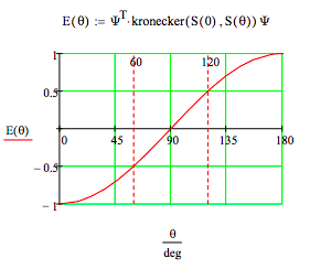
The expectation value as a function of the relative orientation of the detectors reveals the level of correlation between the two spin measurements. For θ = 0⁰ there is perfect anti-correlation; for θ = 180⁰ perfect correlation; for θ = 90⁰ no correlation; for θ = 60⁰ intermediate anti-correlation (-0.5) and for θ = 120⁰ intermediate correlation (0.5).

A Quantum Simulation: This thought experiment is simulated using the following quantum circuit. As shown below the results are in agreement with the previous theoretical quantum calculations. The initial Hadamard and CNOT gates create the singlet state from the |11> input. Rz(θ) rotates spin B. The final Hadamard gates prepare the system for measurement. See arXiv:1712.05642v2 for further detail.

\[ \begin{matrix} \text{Spin A} & |1 \rangle & \triangleright & H & \cdot & \cdots & H & \triangleright & \text{Measure 0 or 1: Eigenvalue +1 or -1} \\ ~ & ~ & ~ & ~ & | \\ \text{Spin B} & |1 \rangle & \triangleright & \cdots & \oplus & R_z ( \theta) & H & \triangleright & \text{Measure 0 or 1: Eigenvalue +1 or -1} \end{matrix} \nonumber \]

The quantum gates required to execute this circuit:

\[ \begin{matrix} \text{Identity} & \text{Hadamard gate} & \text{R}_z ~ \text{Rotation} & \text{Controlled NOT} \\ I = \begin{pmatrix} 1 & 0 \\ 0 & 1 \end{pmatrix} & H = \frac{1}{ \sqrt{2}} \begin{pmatrix} 1 & 1 \\ 1 & -1 \end{pmatrix} & R_z ( \theta) = \begin{pmatrix} 1 & 0 \\ 0 & e^{i \theta} \end{pmatrix} & \text{CNOT} = \begin{pmatrix} 1 & 0 & 0 & 0 \\ 0 & 1 & 0 & 0 \\ 0 & 0 & 0 & 1 \\ 0 & 0 & 1 & 0 \end{pmatrix} \end{matrix} \nonumber \]

The operator representing the circuit is constructed from the matrix operators provided above.

\[ \text{Op} (\theta) = \text{kronecker(H, H) kronecker(I, R}_z (\theta)) \text{CNOT kronecker(H, I)} \nonumber \]

There are four equally likely measurement outcomes with the eigenvalues and overall expectation values shown below for relative measurement angles 0 and 120 deg (2π/3).

\[ \begin{array}{r & l} |00 \rangle \text{eigenvalue +1 } \left[ \left| \begin{pmatrix} 1 \\ 0 \\ 0 \\ 0 \end{pmatrix}^T \text{ Op(0 deg)} \begin{pmatrix} 0 \\ 0 \\ 0 \\ 1 \end{pmatrix} \right| \right] ^2 = 0 & |01 \rangle \text{eigenvalue -1 } \left[ \left| \begin{pmatrix} 0 \\ 1 \\ 0 \\ 0 \end{pmatrix}^T \text{ Op(0 deg)} \begin{pmatrix} 0 \\ 0 \\ 0 \\ 1 \end{pmatrix} \right| \right] ^2 = 0.5 \\ |10 \rangle \text{eigenvalue -1 } \left[ \left| \begin{pmatrix} 0 \\ 0 \\ 1 \\ 0 \end{pmatrix}^T \text{ Op(0 deg)} \begin{pmatrix} 0 \\ 0 \\ 0 \\ 1 \end{pmatrix} \right| \right] ^2 = 0.5 & |11 \rangle \text{eigenvalue +1 } \left[ \left| \begin{pmatrix} 0 \\ 0 \\ 0 \\ 1 \end{pmatrix}^T \text{ Op(0 deg)} \begin{pmatrix} 0 \\ 0 \\ 0 \\ 1 \end{pmatrix} \right| \right] ^2 = 0 \\ \text{Expectation value}: & 0 - 0.5 - 0.5 + 0 = -1 \\ |00 \rangle \text{eigenvalue +1 } \left[ \left| \begin{pmatrix} 1 \\ 0 \\ 0 \\ 0 \end{pmatrix}^T \text{ Op \left( \frac{2 \pi}{3} \right)} \begin{pmatrix} 0 \\ 0 \\ 0 \\ 1 \end{pmatrix} \right| \right] ^2 = 0.375 & |01 \rangle \text{eigenvalue -1 } \left[ \left| \begin{pmatrix} 0 \\ 1 \\ 0 \\ 0 \end{pmatrix}^T \text{ \left( \frac{2 \pi}{3} \right)} \begin{pmatrix} 0 \\ 0 \\ 0 \\ 1 \end{pmatrix} \right| \right] ^2 = 0.125 \\ |10 \rangle \text{eigenvalue -1 } \left[ \left| \begin{pmatrix} 0 \\ 0 \\ 1 \\ 0 \end{pmatrix}^T \text{ \left( \frac{2 \pi}{3} \right)} \begin{pmatrix} 0 \\ 0 \\ 0 \\ 1 \end{pmatrix} \right| \right] ^2 = 0.125 & |11 \rangle \text{eigenvalue +1 } \left[ \left| \begin{pmatrix} 0 \\ 0 \\ 0 \\ 1 \end{pmatrix}^T \text{ \left( \frac{2 \pi}{3} \right)} \begin{pmatrix} 0 \\ 0 \\ 0 \\ 1 \end{pmatrix} \right| \right] ^2 = 0.375 \\ \text{Expectation value}: & 0.375 - 0.125 + 0.375 - 0.125 = 0.5 \end{array} \nonumber \]