
8.28: Nonclassial Correlations Revealed with Mermin's Pentagram
- Page ID
- 143739

\( \newcommand{\vecs}[1]{\overset { \scriptstyle \rightharpoonup} {\mathbf{#1}} } \)
\( \newcommand{\vecd}[1]{\overset{-\!-\!\rightharpoonup}{\vphantom{a}\smash {#1}}} \)
\( \newcommand{\id}{\mathrm{id}}\) \( \newcommand{\Span}{\mathrm{span}}\)
( \newcommand{\kernel}{\mathrm{null}\,}\) \( \newcommand{\range}{\mathrm{range}\,}\)
\( \newcommand{\RealPart}{\mathrm{Re}}\) \( \newcommand{\ImaginaryPart}{\mathrm{Im}}\)
\( \newcommand{\Argument}{\mathrm{Arg}}\) \( \newcommand{\norm}[1]{\| #1 \|}\)
\( \newcommand{\inner}[2]{\langle #1, #2 \rangle}\)
\( \newcommand{\Span}{\mathrm{span}}\)
\( \newcommand{\id}{\mathrm{id}}\)
\( \newcommand{\Span}{\mathrm{span}}\)
\( \newcommand{\kernel}{\mathrm{null}\,}\)
\( \newcommand{\range}{\mathrm{range}\,}\)
\( \newcommand{\RealPart}{\mathrm{Re}}\)
\( \newcommand{\ImaginaryPart}{\mathrm{Im}}\)
\( \newcommand{\Argument}{\mathrm{Arg}}\)
\( \newcommand{\norm}[1]{\| #1 \|}\)
\( \newcommand{\inner}[2]{\langle #1, #2 \rangle}\)
\( \newcommand{\Span}{\mathrm{span}}\) \( \newcommand{\AA}{\unicode[.8,0]{x212B}}\)
\( \newcommand{\vectorA}[1]{\vec{#1}} % arrow\)
\( \newcommand{\vectorAt}[1]{\vec{\text{#1}}} % arrow\)
\( \newcommand{\vectorB}[1]{\overset { \scriptstyle \rightharpoonup} {\mathbf{#1}} } \)
\( \newcommand{\vectorC}[1]{\textbf{#1}} \)
\( \newcommand{\vectorD}[1]{\overrightarrow{#1}} \)
\( \newcommand{\vectorDt}[1]{\overrightarrow{\text{#1}}} \)
\( \newcommand{\vectE}[1]{\overset{-\!-\!\rightharpoonup}{\vphantom{a}\smash{\mathbf {#1}}}} \)
\( \newcommand{\vecs}[1]{\overset { \scriptstyle \rightharpoonup} {\mathbf{#1}} } \)
\( \newcommand{\vecd}[1]{\overset{-\!-\!\rightharpoonup}{\vphantom{a}\smash {#1}}} \)
\(\newcommand{\avec}{\mathbf a}\) \(\newcommand{\bvec}{\mathbf b}\) \(\newcommand{\cvec}{\mathbf c}\) \(\newcommand{\dvec}{\mathbf d}\) \(\newcommand{\dtil}{\widetilde{\mathbf d}}\) \(\newcommand{\evec}{\mathbf e}\) \(\newcommand{\fvec}{\mathbf f}\) \(\newcommand{\nvec}{\mathbf n}\) \(\newcommand{\pvec}{\mathbf p}\) \(\newcommand{\qvec}{\mathbf q}\) \(\newcommand{\svec}{\mathbf s}\) \(\newcommand{\tvec}{\mathbf t}\) \(\newcommand{\uvec}{\mathbf u}\) \(\newcommand{\vvec}{\mathbf v}\) \(\newcommand{\wvec}{\mathbf w}\) \(\newcommand{\xvec}{\mathbf x}\) \(\newcommand{\yvec}{\mathbf y}\) \(\newcommand{\zvec}{\mathbf z}\) \(\newcommand{\rvec}{\mathbf r}\) \(\newcommand{\mvec}{\mathbf m}\) \(\newcommand{\zerovec}{\mathbf 0}\) \(\newcommand{\onevec}{\mathbf 1}\) \(\newcommand{\real}{\mathbb R}\) \(\newcommand{\twovec}[2]{\left[\begin{array}{r}#1 \\ #2 \end{array}\right]}\) \(\newcommand{\ctwovec}[2]{\left[\begin{array}{c}#1 \\ #2 \end{array}\right]}\) \(\newcommand{\threevec}[3]{\left[\begin{array}{r}#1 \\ #2 \\ #3 \end{array}\right]}\) \(\newcommand{\cthreevec}[3]{\left[\begin{array}{c}#1 \\ #2 \\ #3 \end{array}\right]}\) \(\newcommand{\fourvec}[4]{\left[\begin{array}{r}#1 \\ #2 \\ #3 \\ #4 \end{array}\right]}\) \(\newcommand{\cfourvec}[4]{\left[\begin{array}{c}#1 \\ #2 \\ #3 \\ #4 \end{array}\right]}\) \(\newcommand{\fivevec}[5]{\left[\begin{array}{r}#1 \\ #2 \\ #3 \\ #4 \\ #5 \\ \end{array}\right]}\) \(\newcommand{\cfivevec}[5]{\left[\begin{array}{c}#1 \\ #2 \\ #3 \\ #4 \\ #5 \\ \end{array}\right]}\) \(\newcommand{\mattwo}[4]{\left[\begin{array}{rr}#1 \amp #2 \\ #3 \amp #4 \\ \end{array}\right]}\) \(\newcommand{\laspan}[1]{\text{Span}\{#1\}}\) \(\newcommand{\bcal}{\cal B}\) \(\newcommand{\ccal}{\cal C}\) \(\newcommand{\scal}{\cal S}\) \(\newcommand{\wcal}{\cal W}\) \(\newcommand{\ecal}{\cal E}\) \(\newcommand{\coords}[2]{\left\{#1\right\}_{#2}}\) \(\newcommand{\gray}[1]{\color{gray}{#1}}\) \(\newcommand{\lgray}[1]{\color{lightgray}{#1}}\) \(\newcommand{\rank}{\operatorname{rank}}\) \(\newcommand{\row}{\text{Row}}\) \(\newcommand{\col}{\text{Col}}\) \(\renewcommand{\row}{\text{Row}}\) \(\newcommand{\nul}{\text{Nul}}\) \(\newcommand{\var}{\text{Var}}\) \(\newcommand{\corr}{\text{corr}}\) \(\newcommand{\len}[1]{\left|#1\right|}\) \(\newcommand{\bbar}{\overline{\bvec}}\) \(\newcommand{\bhat}{\widehat{\bvec}}\) \(\newcommand{\bperp}{\bvec^\perp}\) \(\newcommand{\xhat}{\widehat{\xvec}}\) \(\newcommand{\vhat}{\widehat{\vvec}}\) \(\newcommand{\uhat}{\widehat{\uvec}}\) \(\newcommand{\what}{\widehat{\wvec}}\) \(\newcommand{\Sighat}{\widehat{\Sigma}}\) \(\newcommand{\lt}{<}\) \(\newcommand{\gt}{>}\) \(\newcommand{\amp}{&}\) \(\definecolor{fillinmathshade}{gray}{0.9}\)A source emits the following six cubit state (|0> and |1> are orthogonal states), with cubits 1,3 and 5 going to Alice, and cubits 2, 4 and 6 going to Bob. This example is due to P. K. Aravind and available at arXiv:quant-ph/0701031v1.
\[ | \Psi \rangle = \frac{1}{ \sqrt{2}} (| 0 \rangle_1 |0 \rangle_2 + |1 \rangle_1 |1 \rangle_2 ) \otimes \frac{1}{ \sqrt{2}} ( |0 \rangle_3 |0 \rangle_4 + |1 \rangle_3 |1 \rangle_4 ) \otimes \frac{1}{ \sqrt{2}} (|0 \rangle_5 |0 \rangle_6 + |1 \rangle_5 |1 \rangle_6) = \frac{1}{ 2 \sqrt{2}} \begin{bmatrix} |0 \rangle_1 |0 \rangle_2 |0 \rangle_3 |0 \rangle_4 |0 \rangle_5 |0 \rangle_6 + |0 \rangle_1 |0 \rangle_2 |1 \rangle_3 |1 \rangle_4 |0 \rangle_5 |0 \rangle_6 + |1 \rangle_1 |1 \rangle_2 |0 \rangle_3 |0 \rangle_4 |0 \rangle_5 |0 \rangle_6 + |1 \rangle_1 |1 \rangle_2 |1 \rangle_3 |1 \rangle_4 |0 \rangle_5 |0 \rangle_6 \\ |0 \rangle_1 |0 \rangle_2 |0 \rangle_3 |0 \rangle_4 |1 \rangle_5 |1 \rangle_6 + |0 \rangle_1 |0 \rangle_2 |1 \rangle_3 |1 \rangle_4 |1 \rangle_5 |1 \rangle_6 + |1 \rangle_1 |1 \rangle_2 |0 \rangle_3 |0 \rangle_4 |1 \rangle_5 |1 \rangle_6 + |1 \rangle_1 |1 \rangle_2 |1 \rangle_3 |1 \rangle_4 |1 \rangle_5 |1 \rangle_6 \end{bmatrix} \nonumber \]
Ψ can be written in condensed binary format as,
\[ | \Psi \rangle = \frac{1}{ 2 \sqrt{2}} \left[ |000000 \rangle + |001100 \rangle + |110000 \rangle + |111100 \rangle + |000011 \rangle + |001111 \rangle + |110011 \rangle +|111111 \rangle \right] \nonumber \]
In decimal notation the kets contain 0, 12, 48, 60, 3, 15, 51, and 63. All other vector elements are zero.
\[ \begin{matrix} i = 0 ... 63 & \Psi_i = 0 \end{matrix} \nonumber \]
\[ \begin{matrix} \Psi_0 = \frac{1}{ 2 \sqrt{2}} & \Psi_3 = \frac{1}{2 \sqrt{2}} & \Psi_{12} = \frac{1}{2 \sqrt{2}} & \Psi_{15} = \frac{1}{2 \sqrt{2}} \\ \Psi_{48} = \frac{1}{2 \sqrt{2}} & \Psi_{51} = \frac{1}{2 \sqrt{2}} & \Psi_{60} = \frac{1}{2 \sqrt{2}} & \Psi_{63} = \frac{1}{2 \sqrt{2}} \end{matrix} \nonumber \]
The following pentagram describes the measurement protocols followed by Alice and Bob.
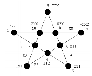
Alice and Bob independently and randomly select one of five measurement protocols (E1, E2, E3, E4 and E5) shown on the edges of the pentagram above each time the source emits the entangled particles, and record the result (+1 or -1) for each vertex. After a statistically meaningful number of events they compare their results.
Each vertex represents a three qubit measurement sequence shown above and given in the following table. Note that Alice's sequence uses the identity operator for photons 2, 4 and 6 because she receives photons 1, 3 and 5, while Bob uses the identity operator for photons 1, 3 and 5 because he receives photons 2, 4 and 6.
\[ \begin{pmatrix} \text{Operator} & \text{Alice} & \text{Bob} \\ 1 & A( - \sigma_z,~ I,~ \sigma_z,~I,~ \sigma_z,~I) & B(I,~ - \sigma_z,~I,~ \sigma_z,~I,~ \sigma_z) \\ 2 & A( \sigma_z,~ I,~ I,~I,~ I,~I) & B(I,~ \sigma_z,~I,~ I,~I,~ I) \\ 3 & A( I,~ I,~ \sigma_x,~I,~ I,~I) & B(I,~ I,~I,~ \sigma_x,~I,~ I) \\ 4 & A(I,~ I,~ I,~I,~ \sigma_z,~I) & B(I,~ I,~I,~ I,~I,~ \sigma_z) \\ 5 & A(I,~ I,~ \sigma_z,~I,~ I,~I) & B(I,~ I,~I,~ \sigma_z,~I,~ I) \\ 6 & A( \sigma_x,~ I,~ I,~I,~ I,~I) & B(I,~ \sigma_x,~I,~ I,~I,~ I) \\ 7 & A( - \sigma_x,~ I,~ \sigma_x,~I,~ \sigma_x,~I) & B(I,~ - \sigma_x,~I,~ \sigma_x,~I,~ \sigma_z) \\ 8 & A( - \sigma_x,~ I,~ \sigma_z,~I,~ \sigma_x,~I) & B(I,~ - \sigma_x,~I,~ \sigma_z,~I,~ \sigma_x) \\ 9 & A(I,~ I,~ I,~I,~ \sigma_x,~I) & B(I,~ I,~I,~ I,~I,~ \sigma_x) \\ 10 & A( - \sigma_z,~ I,~ \sigma_x,~I,~ \sigma_x,~I) & B(I,~ - \sigma_z,~I,~ \sigma_x,~I,~ \sigma_x) \\ \end{pmatrix} \nonumber \]
The measurement operators required are:
\[ \begin{matrix} I = \begin{pmatrix} 1 & 0 \\ 0 & 1 \end{pmatrix} & \sigma_x = \begin{pmatrix} 0 & 1 \\ 1 & 0 \end{pmatrix} & \sigma_z = \begin{pmatrix} 1 & 0 \\ 0 & -1 \end{pmatrix} & \text{eigenvals}( \sigma_x) = \begin{pmatrix} 1 \\ -1 \end{pmatrix} & \text{eigenvals} ( \sigma_z) = \begin{pmatrix} 1 \\ -1 \end{pmatrix} \end{matrix} \nonumber \]
\[ \begin{matrix} \text{A(a, b, c, d, e, f)} = \text{kronecker(a, kronecker(b, kronecker(c, kronecker(d, kronecker(e, f)))))} \\ \text{B(a, b, c, d, e, f)} = \text{kronecker(a, kronecker(b, kronecker(c, kronecker(d, kronecker(e, f)))))} \end{matrix} \nonumber \]
The eigenvalues of the Pauli operators are +/- 1. The first thing to note is that the individual vertices (measurement sites) flash +1 and -1 one randomly giving expectation values of zero at each vertex.
\[ \begin{pmatrix} \Psi^T A( - \sigma_z,~ I,~ \sigma_z,~I,~ \sigma_z,~I) \Psi & \Psi^T B(I,~ - \sigma_z,~I,~ \sigma_z,~I,~ \sigma_z) \Psi \\ \Psi^T A( \sigma_z,~ I,~ I,~I,~ I,~I) \Psi & \Psi^T B(I,~ \sigma_z,~I,~ I,~I,~ I) \Psi \\ \Psi^T A( I,~ I,~ \sigma_x,~I,~ I,~I) \Psi & \Psi^T B(I,~ I,~I,~ \sigma_x,~I,~ I) \Psi \\ \Psi^T A(I,~ I,~ I,~I,~ \sigma_z,~I) \Psi & \Psi^T B(I,~ I,~I,~ I,~I,~ \sigma_z) \Psi \\ \Psi^T A(I,~ I,~ \sigma_z,~I,~ I,~I) \Psi & \Psi^T B(I,~ I,~I,~ \sigma_z,~I,~ I) \Psi \\ \Psi^T A( \sigma_x,~ I,~ I,~I,~ I,~I) \Psi & \Psi^T B(I,~ \sigma_x,~I,~ I,~I,~ I) \Psi \\ \Psi^T A( - \sigma_x,~ I,~ \sigma_x,~I,~ \sigma_x,~I) \Psi & \Psi^T B(I,~ - \sigma_x,~I,~ \sigma_x,~I,~ \sigma_z) \Psi \\ \Psi^T A( - \sigma_x,~ I,~ \sigma_z,~I,~ \sigma_x,~I) \Psi & \Psi^T B(I,~ - \sigma_x,~I,~ \sigma_z,~I,~ \sigma_x) \Psi \\ \Psi^T A(I,~ I,~ I,~I,~ \sigma_x,~I) \Psi & \Psi^T B(I,~ I,~I,~ I,~I,~ \sigma_x) \Psi \\ \Psi^T A( - \sigma_z,~ I,~ \sigma_x,~I,~ \sigma_x,~I) \Psi & \Psi^T B(I,~ - \sigma_z,~I,~ \sigma_x,~I,~ \sigma_x) \Psi \end{pmatrix} = \begin{pmatrix} 0 & 0 \\ 0 & 0 \\ 0 & 0 \\ 0 & 0 \\ 0 & 0 \\ 0 & 0 \\ 0 & 0 \\ 0 & 0 \\ 0 & 0 \\ 0 & 0 \end{pmatrix} \nonumber \]
However, if Alice and Bob chose the same measurement protocol they always get the same eigenvalue, as is shown by the calculations below.
\[ \begin{pmatrix} \Psi^T A( - \sigma_z,~ I,~ \sigma_z,~I,~ \sigma_z,~I) \Psi & \Psi^T B(I,~ - \sigma_z,~I,~ \sigma_z,~I,~ \sigma_z) \Psi \\ \Psi^T A( \sigma_z,~ I,~ I,~I,~ I,~I) \Psi & \Psi^T B(I,~ \sigma_z,~I,~ I,~I,~ I) \Psi \\ \Psi^T A( I,~ I,~ \sigma_x,~I,~ I,~I) \Psi & \Psi^T B(I,~ I,~I,~ \sigma_x,~I,~ I) \Psi \\ \Psi^T A(I,~ I,~ I,~I,~ \sigma_z,~I) \Psi & \Psi^T B(I,~ I,~I,~ I,~I,~ \sigma_z) \Psi \\ \Psi^T A(I,~ I,~ \sigma_z,~I,~ I,~I) \Psi & \Psi^T B(I,~ I,~I,~ \sigma_z,~I,~ I) \Psi \\ \Psi^T A( \sigma_x,~ I,~ I,~I,~ I,~I) \Psi & \Psi^T B(I,~ \sigma_x,~I,~ I,~I,~ I) \Psi \\ \Psi^T A( - \sigma_x,~ I,~ \sigma_x,~I,~ \sigma_x,~I) \Psi & \Psi^T B(I,~ - \sigma_x,~I,~ \sigma_x,~I,~ \sigma_z) \Psi \\ \Psi^T A( - \sigma_x,~ I,~ \sigma_z,~I,~ \sigma_x,~I) \Psi & \Psi^T B(I,~ - \sigma_x,~I,~ \sigma_z,~I,~ \sigma_x) \Psi \\ \Psi^T A(I,~ I,~ I,~I,~ \sigma_x,~I) \Psi & \Psi^T B(I,~ I,~I,~ I,~I,~ \sigma_x) \Psi \\ \Psi^T A( - \sigma_z,~ I,~ \sigma_x,~I,~ \sigma_x,~I) \Psi & \Psi^T B(I,~ - \sigma_z,~I,~ \sigma_x,~I,~ \sigma_x) \Psi \end{pmatrix} = \begin{pmatrix} 1 \\ 1 \\ 1 \\ 1 \\ 1 \\ 1 \\ 1 \\ 1 \\ 1 \\ 1 \end{pmatrix} \nonumber \]
This result is somewhat surprising given the result immediately above. It suggests (at this point) that the particles involved in this experiment carry instruction sets telling the detectors how to operate, and that Alice and Bob's detectors receive the same sets of instructions.
The edges (E1 through E5) shown on the pentagram identify a sequence of four mutually commuting operators (see Appendix). The net eigenvalues for these sequences of measurements for Alice and Bob are now calculated.
\[ \begin{pmatrix} \Psi^T A( - \sigma_z,~ I,~ \sigma_z,~I,~ \sigma_z,~I) A( \sigma_z,~ I,~ I,~I,~ I,~I) A( I,~ I,~ I,~I,~ \sigma_z,~I) A(I,~ I,~ \sigma_z,~I,~ I,~I) \Psi \\ \Psi^T A(I,~ I,~ \sigma_x,~I,~ I,~I) A(I,~ I,~ I,~I,~ \sigma_z,~I) A( \sigma_x,~ I,~ I,~I,~ I,~I) A( -\sigma_x,~ I,~ \sigma_x,~I,~ \sigma_z,~I) \Psi \\ \Psi^T A(I,~ I,~ \sigma_x,~I,~ I,~I) A( \sigma_x,~ I,~ I,~I,~ I,~I) A( - \sigma_x,~ I,~ \sigma_x,~I,~ \sigma_x,~I) A(I,~ I,~ I,~I,~ \sigma_x,~I) \Psi \\ \Psi^T A(I,~ I,~ \sigma_z,~I,~ I,~I) A( \sigma_x,~ I,~ I,~I,~ I,~I) A( - \sigma_x,~ I,~ \sigma_z,~I,~ \sigma_x,~I) A(I,~ I,~ I,~I,~ \sigma_x,~I) \Psi \\ \Psi^T A(- \sigma_z,~ I,~ \sigma_z,~I,~ \sigma_z,~I) A( \sigma_z,~ I,~ \sigma_x,~I,~ \sigma_x,~I) A( - \sigma_x,~ I,~ \sigma_z,~I,~ \sigma_x,~I) A(- \sigma_x,~ I,~ \sigma_x,~I,~ \sigma_z,~I) \Psi \\ \end{pmatrix} = \begin{pmatrix} -1 \\ -1 \\ -1 \\ -1 \\ -1 \end{pmatrix} \nonumber \]
\[ \begin{pmatrix} \Psi^T B(I,~ - \sigma_z,~I,~ \sigma_z,~I,~ \sigma_z) & B(I,~ \sigma_z,~I,~I,~I,~I) & B(I,~I,~I,~I,~I,~ \sigma_z) & B(I,~I,~I,~ \sigma_z,~I,~I) \\ \Psi^T B(I,~I,~I,~ \sigma_x,~I,~I) & B(I,~I,~I,~I,~I,~ \sigma_z) & B(I,~ \sigma_x,~I,~I,~I,~I) & B(I,~ - \sigma_x,~I,~ \sigma_x,~I,~ \sigma_z) \\ \Psi^T B(I,~I,~I,~ \sigma_x,~I,~I) & B(I,~ \sigma_z,~I,~I,~I,~I) & B(I,~ - \sigma_z,~I,~ \sigma_z,~I,~ \sigma_x) & B(I,~ I,~I,~ I,~I,~ \sigma_x) \\ \Psi^T B(I,~I,~I,~ \sigma_z,~I,~I) & B(I,~ \sigma_x,~I,~I,~I,~I) & B(I,~ - \sigma_x,~I,~ \sigma_z,~I,~ \sigma_x) & B(I,~ I,~I,~ I,~I,~ \sigma_x) \\ \Psi^T B(I,~ - \sigma_z,~I,~ \sigma_z,~I,~ \sigma_z) & B(I,~ - \sigma_z,~I,~ \sigma_x,~I,~ \sigma_x) & B(I,~ - \sigma_x,~I,~ \sigma_z,~I,~ \sigma_x) & B(I,~ - \sigma_x,~I,~ \sigma_x,~I,~ \sigma_z) \\ \end{pmatrix} \begin{pmatrix} -1 \\ -1 \\ -1 \\ -1 \\ -1 \end{pmatrix} \nonumber \]
We now have the problem of reconciling these results with those immediately prior. How is it possible to assign +1s and -1s to the measurement vertices such that they satisfy the results immediately above. The answer is that it is not possible. The ideas of instruction sets and elements of reality are not capable of explaining these results.
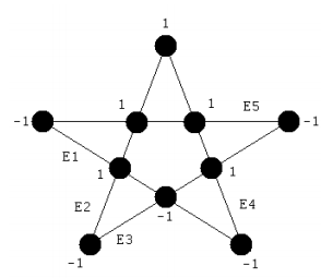
For this assignment of vertex eigenvalues we see that the composite eigenvalue (-1) is satisfied for E1, E2, E3 and E4, but is violated for E5. All attempts to assign +/-1 values to the vertices fail to satisfy the composite eigenvalue for one of the measurement protocols.
Appendix
The four operators comprising the five measurement protocols mutually commute. This is demonstrated below for the E1 protocol.
\[ \begin{matrix} ( - \sigma_z \sigma_z \sigma_z ) ( \sigma_z \text{I I} ) - (\sigma_z \text{I I})( -\sigma_z \sigma_z \sigma_z) = \begin{pmatrix} 0 & 0 \\ 0 & 0 \end{pmatrix} & ( - \sigma_z \sigma_z \sigma_z ) (\text{I I} \sigma_z) - (\text{I I} \sigma_z)( -\sigma_z \sigma_z \sigma_z) = \begin{pmatrix} 0 & 0 \\ 0 & 0 \end{pmatrix} \\ ( - \sigma_z \sigma_z \sigma_z ) (\text{I} \sigma_z \text{I} ) - (\text{I} \sigma_z \text{I})( -\sigma_z \sigma_z \sigma_z) = \begin{pmatrix} 0 & 0 \\ 0 & 0 \end{pmatrix} & ( \sigma_z \text{I I}) (\text{I I} \sigma_z) - (\text{I I} \sigma_z)( \sigma_z \text{I I}) = \begin{pmatrix} 0 & 0 \\ 0 & 0 \end{pmatrix} \\ ( \sigma_z \text{I I}) (\text{I} \sigma_z \text{I} ) - (\text{I} \sigma_z \text{I})( \sigma_z \text{I I}) = \begin{pmatrix} 0 & 0 \\ 0 & 0 \end{pmatrix} & ( \text{I I} \sigma_z) (\text{I} \sigma_z \text{I}) - (\text{I} \sigma_z \text{I})( \text{I I} \sigma_z) = \begin{pmatrix} 0 & 0 \\ 0 & 0 \end{pmatrix} \end{matrix} \nonumber \]
It is also the case that the measurement protocols commute. This is demonstrated for E1 and E5.
\[ \left[ ( - \sigma_z \sigma_z \sigma_z) (\sigma_z \text{I I} ( \text{I I} \sigma_z) ( \text{I} \sigma_z \text{I}) \right] \left[ ( - \sigma_z \sigma_z \sigma_z ) (- \sigma_z \sigma_x \sigma_x ) ( - \sigma_x \sigma_z \sigma_x )( - \sigma_x \sigma_x \sigma_z) \right] ... + - \left[ ( -\sigma_z \sigma_z \sigma_z) ( - \sigma_z \sigma_x \sigma_x) ( -\sigma_x \sigma_z \sigma_x) ( - \sigma_x \sigma_x \sigma_z ) \right] \left[ ( - \sigma_z \sigma_z \sigma_z) ( \sigma_z \text{I I}) ( \text{I I} \sigma_z) ( \text{I} \sigma_z \text{I}) \right] = \begin{pmatrix} 0 & 0 \\ 0 & 0 \end{pmatrix} \nonumber \]