
22.3.4: iv. Review Exercise Solutions
- Page ID
- 81686

\( \newcommand{\vecs}[1]{\overset { \scriptstyle \rightharpoonup} {\mathbf{#1}} } \)
\( \newcommand{\vecd}[1]{\overset{-\!-\!\rightharpoonup}{\vphantom{a}\smash {#1}}} \)
\( \newcommand{\id}{\mathrm{id}}\) \( \newcommand{\Span}{\mathrm{span}}\)
( \newcommand{\kernel}{\mathrm{null}\,}\) \( \newcommand{\range}{\mathrm{range}\,}\)
\( \newcommand{\RealPart}{\mathrm{Re}}\) \( \newcommand{\ImaginaryPart}{\mathrm{Im}}\)
\( \newcommand{\Argument}{\mathrm{Arg}}\) \( \newcommand{\norm}[1]{\| #1 \|}\)
\( \newcommand{\inner}[2]{\langle #1, #2 \rangle}\)
\( \newcommand{\Span}{\mathrm{span}}\)
\( \newcommand{\id}{\mathrm{id}}\)
\( \newcommand{\Span}{\mathrm{span}}\)
\( \newcommand{\kernel}{\mathrm{null}\,}\)
\( \newcommand{\range}{\mathrm{range}\,}\)
\( \newcommand{\RealPart}{\mathrm{Re}}\)
\( \newcommand{\ImaginaryPart}{\mathrm{Im}}\)
\( \newcommand{\Argument}{\mathrm{Arg}}\)
\( \newcommand{\norm}[1]{\| #1 \|}\)
\( \newcommand{\inner}[2]{\langle #1, #2 \rangle}\)
\( \newcommand{\Span}{\mathrm{span}}\) \( \newcommand{\AA}{\unicode[.8,0]{x212B}}\)
\( \newcommand{\vectorA}[1]{\vec{#1}} % arrow\)
\( \newcommand{\vectorAt}[1]{\vec{\text{#1}}} % arrow\)
\( \newcommand{\vectorB}[1]{\overset { \scriptstyle \rightharpoonup} {\mathbf{#1}} } \)
\( \newcommand{\vectorC}[1]{\textbf{#1}} \)
\( \newcommand{\vectorD}[1]{\overrightarrow{#1}} \)
\( \newcommand{\vectorDt}[1]{\overrightarrow{\text{#1}}} \)
\( \newcommand{\vectE}[1]{\overset{-\!-\!\rightharpoonup}{\vphantom{a}\smash{\mathbf {#1}}}} \)
\( \newcommand{\vecs}[1]{\overset { \scriptstyle \rightharpoonup} {\mathbf{#1}} } \)
\( \newcommand{\vecd}[1]{\overset{-\!-\!\rightharpoonup}{\vphantom{a}\smash {#1}}} \)
\(\newcommand{\avec}{\mathbf a}\) \(\newcommand{\bvec}{\mathbf b}\) \(\newcommand{\cvec}{\mathbf c}\) \(\newcommand{\dvec}{\mathbf d}\) \(\newcommand{\dtil}{\widetilde{\mathbf d}}\) \(\newcommand{\evec}{\mathbf e}\) \(\newcommand{\fvec}{\mathbf f}\) \(\newcommand{\nvec}{\mathbf n}\) \(\newcommand{\pvec}{\mathbf p}\) \(\newcommand{\qvec}{\mathbf q}\) \(\newcommand{\svec}{\mathbf s}\) \(\newcommand{\tvec}{\mathbf t}\) \(\newcommand{\uvec}{\mathbf u}\) \(\newcommand{\vvec}{\mathbf v}\) \(\newcommand{\wvec}{\mathbf w}\) \(\newcommand{\xvec}{\mathbf x}\) \(\newcommand{\yvec}{\mathbf y}\) \(\newcommand{\zvec}{\mathbf z}\) \(\newcommand{\rvec}{\mathbf r}\) \(\newcommand{\mvec}{\mathbf m}\) \(\newcommand{\zerovec}{\mathbf 0}\) \(\newcommand{\onevec}{\mathbf 1}\) \(\newcommand{\real}{\mathbb R}\) \(\newcommand{\twovec}[2]{\left[\begin{array}{r}#1 \\ #2 \end{array}\right]}\) \(\newcommand{\ctwovec}[2]{\left[\begin{array}{c}#1 \\ #2 \end{array}\right]}\) \(\newcommand{\threevec}[3]{\left[\begin{array}{r}#1 \\ #2 \\ #3 \end{array}\right]}\) \(\newcommand{\cthreevec}[3]{\left[\begin{array}{c}#1 \\ #2 \\ #3 \end{array}\right]}\) \(\newcommand{\fourvec}[4]{\left[\begin{array}{r}#1 \\ #2 \\ #3 \\ #4 \end{array}\right]}\) \(\newcommand{\cfourvec}[4]{\left[\begin{array}{c}#1 \\ #2 \\ #3 \\ #4 \end{array}\right]}\) \(\newcommand{\fivevec}[5]{\left[\begin{array}{r}#1 \\ #2 \\ #3 \\ #4 \\ #5 \\ \end{array}\right]}\) \(\newcommand{\cfivevec}[5]{\left[\begin{array}{c}#1 \\ #2 \\ #3 \\ #4 \\ #5 \\ \end{array}\right]}\) \(\newcommand{\mattwo}[4]{\left[\begin{array}{rr}#1 \amp #2 \\ #3 \amp #4 \\ \end{array}\right]}\) \(\newcommand{\laspan}[1]{\text{Span}\{#1\}}\) \(\newcommand{\bcal}{\cal B}\) \(\newcommand{\ccal}{\cal C}\) \(\newcommand{\scal}{\cal S}\) \(\newcommand{\wcal}{\cal W}\) \(\newcommand{\ecal}{\cal E}\) \(\newcommand{\coords}[2]{\left\{#1\right\}_{#2}}\) \(\newcommand{\gray}[1]{\color{gray}{#1}}\) \(\newcommand{\lgray}[1]{\color{lightgray}{#1}}\) \(\newcommand{\rank}{\operatorname{rank}}\) \(\newcommand{\row}{\text{Row}}\) \(\newcommand{\col}{\text{Col}}\) \(\renewcommand{\row}{\text{Row}}\) \(\newcommand{\nul}{\text{Nul}}\) \(\newcommand{\var}{\text{Var}}\) \(\newcommand{\corr}{\text{corr}}\) \(\newcommand{\len}[1]{\left|#1\right|}\) \(\newcommand{\bbar}{\overline{\bvec}}\) \(\newcommand{\bhat}{\widehat{\bvec}}\) \(\newcommand{\bperp}{\bvec^\perp}\) \(\newcommand{\xhat}{\widehat{\xvec}}\) \(\newcommand{\vhat}{\widehat{\vvec}}\) \(\newcommand{\uhat}{\widehat{\uvec}}\) \(\newcommand{\what}{\widehat{\wvec}}\) \(\newcommand{\Sighat}{\widehat{\Sigma}}\) \(\newcommand{\lt}{<}\) \(\newcommand{\gt}{>}\) \(\newcommand{\amp}{&}\) \(\definecolor{fillinmathshade}{gray}{0.9}\)Q1
a. For non-degenerate point groups one can simply multiply the representations (since only one representation will be obtained):
\[ a_1 \otimes b_1 = b_1 \nonumber \]
Constructing a "box" in this case is unnecessary since it would only contain a single row. Two unpaired electrons will result in a singlet (S=0, \(M_S\)=0), and three triplets (S=1, \(M_S\)=1, S=1, \(M_S\)=0, S=1, \(M_S=-1\)). The states will be: \(^3B_1(M_S\)=1), \(^3B_1(M_S=0\)), (^3B_1(M_S=-1\)), and \(^1B_1(M_S=0\)).
b. Remember that when coupling non-equivalent linear molecule angular momenta, one simple adds the individual Lz values and vector couples the electron spin. So, in this case \((1\pi_u^12\pi_u^1)\), we have \(M_L\) values of 1+1, 1-1, -1+1, and -1-1 (2,0,0, and -2). The term symbol \(\Delta\) is used to denote the spatially doubly degenerate level \((M_L = \pm 2\)) and there are two distinct spatially non-degenerate levels denote by the term symbol \(\sum (M_L=0).\) Again, two unpaired electrons will result in a singlet (\(S=0 \text{, } M_S=0\)), and three triplets \((S=1\text{, } M_S=1\text{; } S=1 \text{, } M_S=0 \text{; } S=1 \text{, } M_S=-1\)). The states generate are then:
\[ ^1\Delta \text{ }(M_L=2) \text{; one states } (M_S=0), \nonumber \]
\[ ^1\Delta \text{ }(M_L=-2) \text{; one states } (M_S=0), \nonumber \]
\[ ^3\Delta \text{ }(M_L=2) \text{; one states } (M_S=\text{1, 0, and -1),} \nonumber \]
\[ ^3\Delta \text{ }(M_L=-2) \text{; one states } (M_S=\text{1, 0, and -1),} \nonumber \]
\[ ^1\Delta \text{ }(M_L=0) \text{; one states } (M_S=0), \nonumber \]
\[ ^1\Delta \text{ }(M_L=0) \text{; one states } (M_S=0), \nonumber \]
\[ ^3\Delta \text{ }(M_L=0) \text{; one states } (M_S=\text{1, 0, and -1), and } \nonumber \]
\[ ^3\Delta \text{ }(M_L=0) \text{; one states } (M_S=\text{1, 0, and -1)} \nonumber \]
c. Constructing the "box" for two equivalent \(\pi\) electrons one obtains:
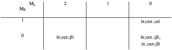
From this "box" one obtains six states:
\[ ^1\Delta (M_L=2)\text{; one state }(M_S=0), \nonumber \]
\[ ^1\Delta (M_L=-2)\text{; one state }(M_S=0), \nonumber \]
\[ ^1\Delta (M_L=0)\text{; one state }(M_S=0), \nonumber \]
\[ ^3\Delta (M_L=0)\text{; three states }(M_S=\text{1, 0, and -1}), \nonumber \]
d. It is not necessary to construct a "box" when coupling non-equivalent angular momenta since the vector coupling results in a range from the sum of the two individual angular momenta to the absolute value of their difference. In this case, \(3d^14d^1\), L=4, 3, 2, 1, 0, and S=1, 0. The term symbol are: \(^3G, ^1G, ^3F, ^1F, ^3D, ^1D, ^3P, ^1P, ^3S\text{, and } ^1S.\) THe L and S angular momenta can be vector coupled to produce further splitting into levels:
\[ \text{ J = L + S ... |L - S|. } \nonumber \]
Denoting J as a term symbol subscript one can identify all the levels and the subsequent (2J + 1) states:
\[ ^3G_5 \text{ (11 states),} \nonumber \]
\[ ^3G_4 \text{ (9 states),} \nonumber \]
\[ ^3G_3 \text{ (7 states),} \nonumber \]
\[ ^1G_4 \text{ (9 states),} \nonumber \]
\[ ^3F_4 \text{ (9 states),} \nonumber \]
\[ ^3F_3 \text{ (7 states),} \nonumber \]
\[ ^3F_2 \text{ (5 states),} \nonumber \]
\[ ^1F_3 \text{ (7 states),} \nonumber \]
\[ ^3D_3 \text{ (7 states),} \nonumber \]
\[ ^3D_2 \text{ (5 states),} \nonumber \]
\[ ^3D_1 \text{ (3 states),} \nonumber \]
\[ ^1D_2 \text{ (5 states),} \nonumber \]
\[ ^3P_2 \text{ (5 states),} \nonumber \]
\[ ^3P_1 \text{ (3 states),} \nonumber \]
\[ ^3P_0 \text{ (1 states),} \nonumber \]
\[ ^1P_1 \text{ (3 states),} \nonumber \]
\[ ^3S_5 \text{ (3 states), and} \nonumber \]
\[ ^1S_0 \text{ (1 states).} \nonumber \]
e. Construction of a "box" for the two equivalent d electrons generates (note the "box" has been turned side ways for convenience):
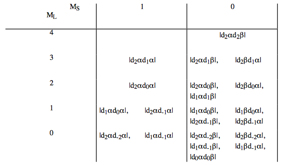
The term symbols are: \(^1G \text{, } ^3F \text{, } ^1D \text{, } ^3P \text{, and } ^1S.\) The L and S angular momenta can be vector coupled to produce further splitting into levels:
\[ ^1G_4 \text{ (9 states),} \nonumber \]
\[ ^3F_4 \text{ (9 states),} \nonumber \]
\[ ^3F_3 \text{ (7 states),} \nonumber \]
\[ ^3F_2 \text{ (5 states),} \nonumber \]
\[ ^1D_2 \text{ (5 states),} \nonumber \]
\[ ^3P_2 \text{ (5 states),} \nonumber \]
\[ ^3P_1 \text{ (3 states),} \nonumber \]
\[ ^3P_0 \text{ (1 states), and} \nonumber \]
\[ ^1S_0 \text{ (1 states).} \nonumber \]