8.3: Mean-Field Models
- Page ID
- 62623
\( \newcommand{\vecs}[1]{\overset { \scriptstyle \rightharpoonup} {\mathbf{#1}} } \)
\( \newcommand{\vecd}[1]{\overset{-\!-\!\rightharpoonup}{\vphantom{a}\smash {#1}}} \)
\( \newcommand{\id}{\mathrm{id}}\) \( \newcommand{\Span}{\mathrm{span}}\)
( \newcommand{\kernel}{\mathrm{null}\,}\) \( \newcommand{\range}{\mathrm{range}\,}\)
\( \newcommand{\RealPart}{\mathrm{Re}}\) \( \newcommand{\ImaginaryPart}{\mathrm{Im}}\)
\( \newcommand{\Argument}{\mathrm{Arg}}\) \( \newcommand{\norm}[1]{\| #1 \|}\)
\( \newcommand{\inner}[2]{\langle #1, #2 \rangle}\)
\( \newcommand{\Span}{\mathrm{span}}\)
\( \newcommand{\id}{\mathrm{id}}\)
\( \newcommand{\Span}{\mathrm{span}}\)
\( \newcommand{\kernel}{\mathrm{null}\,}\)
\( \newcommand{\range}{\mathrm{range}\,}\)
\( \newcommand{\RealPart}{\mathrm{Re}}\)
\( \newcommand{\ImaginaryPart}{\mathrm{Im}}\)
\( \newcommand{\Argument}{\mathrm{Arg}}\)
\( \newcommand{\norm}[1]{\| #1 \|}\)
\( \newcommand{\inner}[2]{\langle #1, #2 \rangle}\)
\( \newcommand{\Span}{\mathrm{span}}\) \( \newcommand{\AA}{\unicode[.8,0]{x212B}}\)
\( \newcommand{\vectorA}[1]{\vec{#1}} % arrow\)
\( \newcommand{\vectorAt}[1]{\vec{\text{#1}}} % arrow\)
\( \newcommand{\vectorB}[1]{\overset { \scriptstyle \rightharpoonup} {\mathbf{#1}} } \)
\( \newcommand{\vectorC}[1]{\textbf{#1}} \)
\( \newcommand{\vectorD}[1]{\overrightarrow{#1}} \)
\( \newcommand{\vectorDt}[1]{\overrightarrow{\text{#1}}} \)
\( \newcommand{\vectE}[1]{\overset{-\!-\!\rightharpoonup}{\vphantom{a}\smash{\mathbf {#1}}}} \)
\( \newcommand{\vecs}[1]{\overset { \scriptstyle \rightharpoonup} {\mathbf{#1}} } \)
\( \newcommand{\vecd}[1]{\overset{-\!-\!\rightharpoonup}{\vphantom{a}\smash {#1}}} \)
\(\newcommand{\avec}{\mathbf a}\) \(\newcommand{\bvec}{\mathbf b}\) \(\newcommand{\cvec}{\mathbf c}\) \(\newcommand{\dvec}{\mathbf d}\) \(\newcommand{\dtil}{\widetilde{\mathbf d}}\) \(\newcommand{\evec}{\mathbf e}\) \(\newcommand{\fvec}{\mathbf f}\) \(\newcommand{\nvec}{\mathbf n}\) \(\newcommand{\pvec}{\mathbf p}\) \(\newcommand{\qvec}{\mathbf q}\) \(\newcommand{\svec}{\mathbf s}\) \(\newcommand{\tvec}{\mathbf t}\) \(\newcommand{\uvec}{\mathbf u}\) \(\newcommand{\vvec}{\mathbf v}\) \(\newcommand{\wvec}{\mathbf w}\) \(\newcommand{\xvec}{\mathbf x}\) \(\newcommand{\yvec}{\mathbf y}\) \(\newcommand{\zvec}{\mathbf z}\) \(\newcommand{\rvec}{\mathbf r}\) \(\newcommand{\mvec}{\mathbf m}\) \(\newcommand{\zerovec}{\mathbf 0}\) \(\newcommand{\onevec}{\mathbf 1}\) \(\newcommand{\real}{\mathbb R}\) \(\newcommand{\twovec}[2]{\left[\begin{array}{r}#1 \\ #2 \end{array}\right]}\) \(\newcommand{\ctwovec}[2]{\left[\begin{array}{c}#1 \\ #2 \end{array}\right]}\) \(\newcommand{\threevec}[3]{\left[\begin{array}{r}#1 \\ #2 \\ #3 \end{array}\right]}\) \(\newcommand{\cthreevec}[3]{\left[\begin{array}{c}#1 \\ #2 \\ #3 \end{array}\right]}\) \(\newcommand{\fourvec}[4]{\left[\begin{array}{r}#1 \\ #2 \\ #3 \\ #4 \end{array}\right]}\) \(\newcommand{\cfourvec}[4]{\left[\begin{array}{c}#1 \\ #2 \\ #3 \\ #4 \end{array}\right]}\) \(\newcommand{\fivevec}[5]{\left[\begin{array}{r}#1 \\ #2 \\ #3 \\ #4 \\ #5 \\ \end{array}\right]}\) \(\newcommand{\cfivevec}[5]{\left[\begin{array}{c}#1 \\ #2 \\ #3 \\ #4 \\ #5 \\ \end{array}\right]}\) \(\newcommand{\mattwo}[4]{\left[\begin{array}{rr}#1 \amp #2 \\ #3 \amp #4 \\ \end{array}\right]}\) \(\newcommand{\laspan}[1]{\text{Span}\{#1\}}\) \(\newcommand{\bcal}{\cal B}\) \(\newcommand{\ccal}{\cal C}\) \(\newcommand{\scal}{\cal S}\) \(\newcommand{\wcal}{\cal W}\) \(\newcommand{\ecal}{\cal E}\) \(\newcommand{\coords}[2]{\left\{#1\right\}_{#2}}\) \(\newcommand{\gray}[1]{\color{gray}{#1}}\) \(\newcommand{\lgray}[1]{\color{lightgray}{#1}}\) \(\newcommand{\rank}{\operatorname{rank}}\) \(\newcommand{\row}{\text{Row}}\) \(\newcommand{\col}{\text{Col}}\) \(\renewcommand{\row}{\text{Row}}\) \(\newcommand{\nul}{\text{Nul}}\) \(\newcommand{\var}{\text{Var}}\) \(\newcommand{\corr}{\text{corr}}\) \(\newcommand{\len}[1]{\left|#1\right|}\) \(\newcommand{\bbar}{\overline{\bvec}}\) \(\newcommand{\bhat}{\widehat{\bvec}}\) \(\newcommand{\bperp}{\bvec^\perp}\) \(\newcommand{\xhat}{\widehat{\xvec}}\) \(\newcommand{\vhat}{\widehat{\vvec}}\) \(\newcommand{\uhat}{\widehat{\uvec}}\) \(\newcommand{\what}{\widehat{\wvec}}\) \(\newcommand{\Sighat}{\widehat{\Sigma}}\) \(\newcommand{\lt}{<}\) \(\newcommand{\gt}{>}\) \(\newcommand{\amp}{&}\) \(\definecolor{fillinmathshade}{gray}{0.9}\)The Mean-Field Model, Which Forms the Basis of Chemists' Pictures of Electronic Structure of Molecules, Is Not Very Accurate
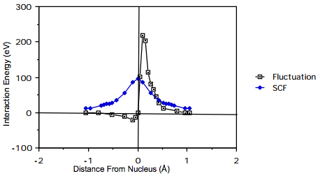
The magnitude and "shape" of such a mean-field potential is shown below for the Beryllium atom. In this figure, the nucleus is at the origin, and one electron is placed at a distance from the nucleus equal to the maximum of the 1s orbital's radial probability density (near 0.13 Å). The radial coordinate of the second is plotted as the abscissa; this second electron is arbitrarily constrained to lie on the line connecting the nucleus and the first electron (along this direction, the inter-electronic interactions are largest). On the ordinate, there are two quantities plotted: (i) the Self-Consistent Field (SCF) mean-field potential \( \int |1s(\textbf{r'})|^2 \frac{e^2}{|\textbf{r}-\textbf{r'}|} \textbf{dr'}\), and (ii) the so-called Fluctuation potential (F), which is the true coulombic \(\frac{e^2}{|\textbf{r}-\textbf{r'}|}\) interaction potential minus the SCF potential.

Figure 8.3.1: Insert caption here!
As a function of the inter-electron distance, the fluctuation potential decays to zero more rapidly than does the SCF potential. For this reason, approaches in which F is treated as a perturbation and corrections to the mean-field picture are computed perturbatively might be expected to be rapidly convergent (whenever perturbations describing long-range interactions arise, convergence of perturbation theory is expected to be slow or not successful). However, the magnitude of F is quite large and remains so over an appreciable range of inter-electron distances. The resultant corrections to
The resultant corrections to the SCF picture are therefore quite large when measured in kcal/mole. For example, the differences \(\Delta E\) between the true (state-of-the-art quantum chemical calculation) energies of interaction among the four electrons in Be and the SCF mean-field estimates of these interactions are given in the table shown below in eV (recall that 1 eV = 23.06 kcal/mole).

Table 8.3.1: Insert caption here!
To provide further insight why the SCF mean-field model in electronic structure theory is of limited accuracy, it can be noted that the average value of the kinetic energy plus the attraction to the Be nucleus plus the SCF interaction potential for one of the 2s orbitals of Be with the three remaining electrons in the \(1s^22s^2\) configuration is:
\[ \langle 2s|\dfrac{-\hbar^2}{2m_e}\nabla^2 - \dfrac{4e^2}{r} + V_{SCF} | 2s \rangle = -15.4 eV; \nonumber \]
the analogous quantity for the 2p orbital in the \(1s^22s^2p\) configuration is:
\[ \langle 2p| \dfrac{-\hbar^2}{2m_e}\nabla^2 - \dfrac{4e^2}{r} + V_{SCF}|2p\rangle = -12.28 eV; \nonumber \]
the corresponding value for the 1s orbital is (negative and) of even larger magnitude. The SCF average coulomb interaction between the two 2s orbitals of \(1s^22s^2\) Be is:
\[ \int |2s(\textbf{r})|^2 |2s(\textbf{r'})|^2 \dfrac{e^2}{|\textbf{r}-\textbf{r'}|} \textbf{dr dr'} = 5,95 eV. \nonumber \]
This data clearly shows that corrections to the SCF model (see the above table) represent significant fractions of the inter-electron interaction energies (e.g., 1.234 eV compared to 5.95- 1.234 = 4.72 eV for the two 2s electrons of Be), and that the interelectron interaction energies, in turn, constitute significant fractions of the total energy of each orbital (e.g., 5.95 -1.234 eV = 4.72 eV out of -15.4 eV for a 2s orbital of Be).
The task of describing the electronic states of atoms and molecules from first principles and in a chemically accurate manner (± 1 kcal/mole) is clearly quite formidable. The orbital picture and its accompanying SCF potential take care of "most" of the interactions among the N electrons (which interact via long-range coulomb forces and whose dynamics requires the application of quantum physics and permutational symmetry). However, the residual fluctuation potential, although of shorter range than the bare coulomb potential, is large enough to cause significant corrections to the mean-field picture. This, in turn, necessitates the use of more sophisticated and computationally taxing techniques (e.g., high order perturbation theory or large variational expansion spaces) to reach the desired chemical accuracy.
Mean-field models are obviously approximations whose accuracy must be determined so scientists can know to what degree they can be "trusted". For electronic structures of atoms and molecules, they require quite substantial corrections to bring them into line with experimental fact. Electrons in atoms and molecules undergo dynamical motions in which their coulomb repulsions cause them to "avoid" one another at every instant of time, not only in the average-repulsion manner that the mean-field models embody. The inclusion of instantaneous spatial correlations among electrons is necessary to achieve a more accurate description of atomic and molecular electronic structure.


