
6.4: Hydrogen Atomic Orbitals Depend upon Three Quantum Numbers
- Page ID
- 13429
- Recognize how the hydrogen atomic orbitals vary as a function of the three primary quantum numbers
The solutions to the hydrogen atom Schrödinger equation discussed previously are functions that are products of a spherical harmonic function and a radial function.
\[ \psi _{n, l, m_l } (r, \theta , \varphi) = \underbrace{R_{n,l} (r)}_{radial} \underbrace{ Y^{m_l}_l (\theta , \varphi)}_{angular} \label {6.1.14} \]
The wavefunctions for the hydrogen atom depend upon the three variables \(r\), \(\theta\), and \(\varphi \) and the three quantum numbers \(n\), \(l\), and \(m_l\). The variables give the position of the electron relative to the proton in spherical coordinates. The absolute square of the wavefunction, \(| \psi (r, \theta , \varphi )|^2\), evaluated at \(r\), \(\theta \), and \(\varphi\) gives the probability density of finding the electron inside a differential volume \(d \tau\), centered at the position specified by \(r\), \(\theta \), and \(\varphi\).
Evaluate the following integrals
- \( \langle \psi (r, \theta, \varphi )| \psi (r, \theta , \varphi ) \rangle \nonumber\)
- \( \langle \psi (r, \theta, \varphi )| \psi (r', \theta' , \varphi' ) \rangle \nonumber\)
- Answer
-
a. This integral is equal to one since \(\psi(r, \theta, \varphi)\) are normalized eigenstates.
b. However, we can explicitly evaluate this integral for any arbitrary pair of eigenstates
\[\begin{align*} \langle\psi(r,\theta,\varphi)|\psi(r',\theta',\varphi')\rangle & = \int\limits_{all space}\psi^*(r,\theta,\varphi)\psi(r',\theta',\varphi')d\tau \\[4pt] &=\int\limits_{0}^{\infty} dr \int\limits_{0}^{\pi}d\theta\int\limits_{0}^{2\pi}d\varphi(r^2\sin(\theta))\overbrace{\psi*(r,\theta,\varphi)}^{R_{n,l}(r)Y_{l}^{m_l}(\theta,\varphi)}\overbrace{\psi(r,\theta,\varphi)}^{R_{n',l'}(r)Y_{l'}^{m'_l}(\theta,\varphi)} \\[4pt] &=\int \limits_{0}^{\infty} dr \int\limits_{0}^{\pi}d\theta \int \limits_{0}^{2\pi} d\varphi(r^2\sin(\theta))[R_{n,l}(r)Y_{l}^{m_l}(\theta,\varphi)][R_{n',l'}(r)Y_{l'}^{m'_l}(\theta,\varphi)] \\[4pt] &=\left[\int\limits_{0}^{\infty}r^2[R_{n,l}(r)R_{n',l'}(r)]dr\right]\left[\int\limits_{0}^{2\pi}\int\limits_{0}^{\pi}\sin(\theta)[Y_{l}^{m_l}(\theta,\varphi)Y_{l'}^{m'_l}(\theta,\varphi)]d\theta d\varphi \right] \\[4pt] &=\langle R_{n,l}(r)|R_{n',l'}(r)\rangle\langle Y_{l}^{m_l}(\theta,\varphi)|Y_{l'}^{m'_l}(\theta,\varphi)\rangle \\[4pt] &=(\delta_{nn'}\delta_{ll'})(\delta_{ll'}\delta_{mm'}) =\delta_{nn'}\delta_{ll'}\delta_{mm'} \end{align*} \nonumber \]
While part a demonstrates normality of the eigenstates, part b demonstrates the orthogonality of the eigenstate (and normality too).
The quantum numbers have names:
- \(n\) is called the principal quantum number,
- \(l\) is called the angular momentum quantum number, and
- \(m_l\) is called the magnetic quantum number because the energy in a magnetic field depends upon \(m_l\).
Often \(l\) is called the azimuthal quantum number because it is a consequence of the \(\theta\)-equation, which involves the azimuthal angle \(\Theta \), referring to the angle to the zenith.
Radial Part of the Wavefunction
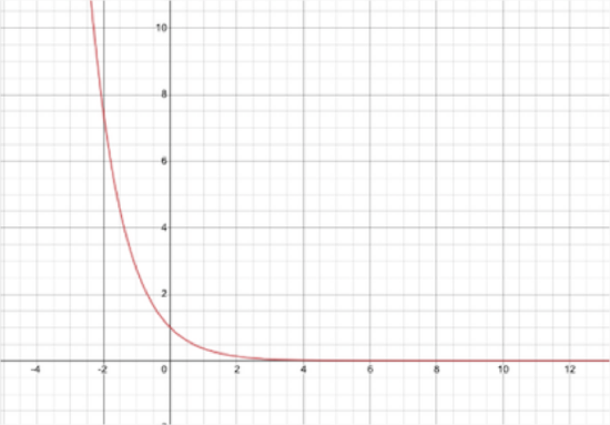
The asymptotic behavior (i.e., far away from the nucleus) to the radial part of the wavefunction is
\[ R_{asymptotic} (r) \sim \exp \left(-\dfrac {r}{n} a_0 \right) \label {6.1.15} \]
where \(n\) will turn out to be a quantum number and \(a_0\) is the Bohr radius (~52.9 pm). Note that this function decreases exponentially with distance, in a manner similar to the decaying exponential portion of the harmonic oscillator wavefunctions, but with a different distance dependence, \(r\) vs. \(r^2\).
What happens to the magnitude of \(R_{asymptotic}(r)\) as the distance \(r\) from the proton approaches infinity? Sketch a graph of the function, \(R_{asymptotic}(r)\). Why might this behavior be expected for an electron in a hydrogen atom?
- Answer
-
\[R(r)=e^{-\frac{c}{n} a_{0}} \nonumber \]
As \(r\) approaches infinity, the exponential decay goes to zero, this is to be expected as the likelihood of an electron being found at an infinite distance away is almost zero too.
The polynomials produced by the truncation of the power series are related to the associated Laguerre polynomials, \(L_n , _l(r)\), where the set of \(c_i\) are constant coefficients.
\[L_{n, l} (r) = \sum _{r=0}^{n-l-1} c_i r^i \label {6.1.16} \]
These polynomials are identified by two indices or quantum numbers, \(n\) and \(l\). Physically acceptable solutions require that \(n\) must be greater than or equal to \(l +1\). The smallest value for \(l\) is zero, so the smallest value for \(n\) is 1. The angular momentum quantum number affects the solution to the radial equation because it appears in the radial differential equation, (Equation \(\ref{6.1.14}\)).
The \(R(r)\) functions that solve the radial differential Equation \(\ref{6.1.14}\), are products of the associated Laguerre polynomials and the exponential factor, multiplied by a normalization factor \((N_{n,l})\) and \(\left (\dfrac {r}{a_0} \right ) ^l\).
\[R (r) = N_{n,l} \left ( \dfrac {r}{a_0} \right ) ^l L_{n,l} (r) e^{-\frac {r}{n {a_0}}} \label {6.1.17} \]
The decreasing exponential term overpowers the increasing polynomial term so that the overall wavefunction exhibits the desired approach to zero at large values of \(r\). The first six radial functions are provided in Table 6.4.1 . Note that the functions in the table exhibit a dependence on \(Z\), the atomic number of the nucleus. As discussed later in this chapter, other one electron systems have electronic states analogous to those for the hydrogen atom, and inclusion of the charge on the nucleus allows the same wavefunctions to be used for all one-electron systems. For hydrogen, \(Z = 1\).
|
|
|
|
|---|---|---|
| 1 | 0 | \(2 \left (\dfrac {Z}{a_0} \right ) ^{3/2} e^{-\rho}\) |
| 2 | 0 | \( \dfrac {1}{2 \sqrt {2}}\left (\dfrac {Z}{a_0} \right ) ^{3/2} (2 - \rho) e^{-\rho/2}\) |
| 2 | 1 | \( \dfrac {1}{2 \sqrt {6}}\left (\dfrac {Z}{a_0} \right ) ^{3/2} \rho e^{-\rho/2}\) |
| 3 | 0 | \( \dfrac {2}{81 \sqrt {3}}\left (\dfrac {Z}{a_0} \right ) ^{3/2} (27 - 18 \rho + 2\rho ^2) e^{-\rho/3}\) |
| 3 | 1 | \( \dfrac {1}{81 \sqrt {6}}\left (\dfrac {Z}{a_0} \right ) ^{3/2} (6 \rho + \rho ^2) e^{-\rho/3}\) |
| 3 | 2 | \( \dfrac {1}{81 \sqrt {30}}\left (\dfrac {Z}{a_0} \right ) ^{3/2} \rho ^2 e^{-\rho/3}\) |
The constraint that \(n\) be greater than or equal to \(l +1\) also turns out to quantize the energy, producing the same quantized expression for hydrogen atom energy levels that was obtained from the Bohr model of the hydrogen atom.
\[ E_n = - \dfrac {\mu e^4}{8 \epsilon ^2_0 h^2 n^2} \nonumber \]
It is interesting to compare the results obtained by solving the Schrödinger equation with Bohr’s model of the hydrogen atom. There are several ways in which the Schrödinger and Bohr models differ.
- First, and perhaps most strikingly, the Schrödinger model does not produce well-defined orbits for the electron. The wavefunctions only give us the probability for the electron to be at various directions and distances from the proton.
- Second, the quantization of angular momentum is different from that proposed by Bohr. Bohr proposed that the angular momentum is quantized in integer units of \(\hbar\), while the Schrödinger model leads to an angular momentum of \( \sqrt{(l (l +1)} \hbar\).
- Third, the quantum numbers appear naturally during solution of the Schrödinger equation while Bohr had to postulate the existence of quantized energy states. Although more complex, the Schrödinger model leads to a better correspondence between theory and experiment over a range of applications that was not possible for the Bohr model.
Explain how the Schrödinger equation leads to the conclusion that the angular momentum of the hydrogen atom can be zero, and explain how the existence of such states with zero angular momentum contradicts Bohr's idea that the electron is orbiting around the proton in the hydrogen atom.
The Three Quantum Numbers
These quantum numbers have specific values that are dictated by the physical constraints or boundary conditions imposed upon the Schrödinger equation: n must be an integer greater than 0, \(l\) can have the values 0 to \(n‑1\), and \(m_l\) can have \(2l + 1\) values ranging from \(-l\) ‑ to \(+l\) in unit or integer steps. The values of the quantum number \(l\) usually are coded by a letter: s means 0, p means 1, d means 2, f means 3; the next codes continue alphabetically (e.g., g means \(l = 4\)). The quantum numbers specify the quantization of physical quantities. The discrete energies of different states of the hydrogen atom are given by n, the magnitude of the angular momentum is given by \(l\), and one component of the angular momentum (usually chosen by chemists to be the z‑component) is given by \(m_l\). The total number of orbitals with a particular value of \(n\) is \(n^2\).
Consider several values for \(n\), and show that the number of orbitals for each \(n\) is \(n^2\).
Construct a table summarizing the allowed values for the quantum numbers \(n\), \(l\), and \(m_l\) for energy levels 1 through 7 of hydrogen.
The notation 3d specifies the quantum numbers for an electron in the hydrogen atom. What are the values for \(n\) and \(l\) ? What are the values for the energy and angular momentum? What are the possible values for the magnetic quantum number? What are the possible orientations for the angular momentum vector?
Contributors and Attributions
David M. Hanson, Erica Harvey, Robert Sweeney, Theresa Julia Zielinski ("Quantum States of Atoms and Molecules")