12.2: Concentration Profiles for Some Simple Mechanisms
- Page ID
- 84366
\( \newcommand{\vecs}[1]{\overset { \scriptstyle \rightharpoonup} {\mathbf{#1}} } \)
\( \newcommand{\vecd}[1]{\overset{-\!-\!\rightharpoonup}{\vphantom{a}\smash {#1}}} \)
\( \newcommand{\id}{\mathrm{id}}\) \( \newcommand{\Span}{\mathrm{span}}\)
( \newcommand{\kernel}{\mathrm{null}\,}\) \( \newcommand{\range}{\mathrm{range}\,}\)
\( \newcommand{\RealPart}{\mathrm{Re}}\) \( \newcommand{\ImaginaryPart}{\mathrm{Im}}\)
\( \newcommand{\Argument}{\mathrm{Arg}}\) \( \newcommand{\norm}[1]{\| #1 \|}\)
\( \newcommand{\inner}[2]{\langle #1, #2 \rangle}\)
\( \newcommand{\Span}{\mathrm{span}}\)
\( \newcommand{\id}{\mathrm{id}}\)
\( \newcommand{\Span}{\mathrm{span}}\)
\( \newcommand{\kernel}{\mathrm{null}\,}\)
\( \newcommand{\range}{\mathrm{range}\,}\)
\( \newcommand{\RealPart}{\mathrm{Re}}\)
\( \newcommand{\ImaginaryPart}{\mathrm{Im}}\)
\( \newcommand{\Argument}{\mathrm{Arg}}\)
\( \newcommand{\norm}[1]{\| #1 \|}\)
\( \newcommand{\inner}[2]{\langle #1, #2 \rangle}\)
\( \newcommand{\Span}{\mathrm{span}}\) \( \newcommand{\AA}{\unicode[.8,0]{x212B}}\)
\( \newcommand{\vectorA}[1]{\vec{#1}} % arrow\)
\( \newcommand{\vectorAt}[1]{\vec{\text{#1}}} % arrow\)
\( \newcommand{\vectorB}[1]{\overset { \scriptstyle \rightharpoonup} {\mathbf{#1}} } \)
\( \newcommand{\vectorC}[1]{\textbf{#1}} \)
\( \newcommand{\vectorD}[1]{\overrightarrow{#1}} \)
\( \newcommand{\vectorDt}[1]{\overrightarrow{\text{#1}}} \)
\( \newcommand{\vectE}[1]{\overset{-\!-\!\rightharpoonup}{\vphantom{a}\smash{\mathbf {#1}}}} \)
\( \newcommand{\vecs}[1]{\overset { \scriptstyle \rightharpoonup} {\mathbf{#1}} } \)
\( \newcommand{\vecd}[1]{\overset{-\!-\!\rightharpoonup}{\vphantom{a}\smash {#1}}} \)
\(\newcommand{\avec}{\mathbf a}\) \(\newcommand{\bvec}{\mathbf b}\) \(\newcommand{\cvec}{\mathbf c}\) \(\newcommand{\dvec}{\mathbf d}\) \(\newcommand{\dtil}{\widetilde{\mathbf d}}\) \(\newcommand{\evec}{\mathbf e}\) \(\newcommand{\fvec}{\mathbf f}\) \(\newcommand{\nvec}{\mathbf n}\) \(\newcommand{\pvec}{\mathbf p}\) \(\newcommand{\qvec}{\mathbf q}\) \(\newcommand{\svec}{\mathbf s}\) \(\newcommand{\tvec}{\mathbf t}\) \(\newcommand{\uvec}{\mathbf u}\) \(\newcommand{\vvec}{\mathbf v}\) \(\newcommand{\wvec}{\mathbf w}\) \(\newcommand{\xvec}{\mathbf x}\) \(\newcommand{\yvec}{\mathbf y}\) \(\newcommand{\zvec}{\mathbf z}\) \(\newcommand{\rvec}{\mathbf r}\) \(\newcommand{\mvec}{\mathbf m}\) \(\newcommand{\zerovec}{\mathbf 0}\) \(\newcommand{\onevec}{\mathbf 1}\) \(\newcommand{\real}{\mathbb R}\) \(\newcommand{\twovec}[2]{\left[\begin{array}{r}#1 \\ #2 \end{array}\right]}\) \(\newcommand{\ctwovec}[2]{\left[\begin{array}{c}#1 \\ #2 \end{array}\right]}\) \(\newcommand{\threevec}[3]{\left[\begin{array}{r}#1 \\ #2 \\ #3 \end{array}\right]}\) \(\newcommand{\cthreevec}[3]{\left[\begin{array}{c}#1 \\ #2 \\ #3 \end{array}\right]}\) \(\newcommand{\fourvec}[4]{\left[\begin{array}{r}#1 \\ #2 \\ #3 \\ #4 \end{array}\right]}\) \(\newcommand{\cfourvec}[4]{\left[\begin{array}{c}#1 \\ #2 \\ #3 \\ #4 \end{array}\right]}\) \(\newcommand{\fivevec}[5]{\left[\begin{array}{r}#1 \\ #2 \\ #3 \\ #4 \\ #5 \\ \end{array}\right]}\) \(\newcommand{\cfivevec}[5]{\left[\begin{array}{c}#1 \\ #2 \\ #3 \\ #4 \\ #5 \\ \end{array}\right]}\) \(\newcommand{\mattwo}[4]{\left[\begin{array}{rr}#1 \amp #2 \\ #3 \amp #4 \\ \end{array}\right]}\) \(\newcommand{\laspan}[1]{\text{Span}\{#1\}}\) \(\newcommand{\bcal}{\cal B}\) \(\newcommand{\ccal}{\cal C}\) \(\newcommand{\scal}{\cal S}\) \(\newcommand{\wcal}{\cal W}\) \(\newcommand{\ecal}{\cal E}\) \(\newcommand{\coords}[2]{\left\{#1\right\}_{#2}}\) \(\newcommand{\gray}[1]{\color{gray}{#1}}\) \(\newcommand{\lgray}[1]{\color{lightgray}{#1}}\) \(\newcommand{\rank}{\operatorname{rank}}\) \(\newcommand{\row}{\text{Row}}\) \(\newcommand{\col}{\text{Col}}\) \(\renewcommand{\row}{\text{Row}}\) \(\newcommand{\nul}{\text{Nul}}\) \(\newcommand{\var}{\text{Var}}\) \(\newcommand{\corr}{\text{corr}}\) \(\newcommand{\len}[1]{\left|#1\right|}\) \(\newcommand{\bbar}{\overline{\bvec}}\) \(\newcommand{\bhat}{\widehat{\bvec}}\) \(\newcommand{\bperp}{\bvec^\perp}\) \(\newcommand{\xhat}{\widehat{\xvec}}\) \(\newcommand{\vhat}{\widehat{\vvec}}\) \(\newcommand{\uhat}{\widehat{\uvec}}\) \(\newcommand{\what}{\widehat{\wvec}}\) \(\newcommand{\Sighat}{\widehat{\Sigma}}\) \(\newcommand{\lt}{<}\) \(\newcommand{\gt}{>}\) \(\newcommand{\amp}{&}\) \(\definecolor{fillinmathshade}{gray}{0.9}\)To illustrate how mechanisms may affect the concentration profile for a reaction, we can examine some simple mechanisms
\(A \rightarrow B\)
In this type of reaction, one substance is simply converting into another. An example of this type of reaction might be the isomerization of methylisocyanide to form acetonitrile (methylcyanide) (Redmon, Purvis, & Bartlett, 1978). If the reaction mechanism consists of a single unimolecular step, which is characterized by the rate constant \(k_1\):
\[ A \xrightarrow{k_1} B \nonumber \]
then rate of change of the concentrations of \(A\) and \(B\) may be written
\[\dfrac{d[A]}{dt} = - k_1 [A] \nonumber \]
and
\[\dfrac{d[B]}{dt} = + k_1 [A] \nonumber \]
A plot the concentrations as a function of time would look as follows:
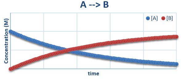
It can be easily seen that the concentration of the reactant (A) decreases as time moves forward, and that of the product (B) increases. This will continue until reactant A is depleted.
\(A \rightleftharpoons B\)
When the system can establish equilibrium, the rate of change of the concentration of A and B will depend on both the forward and reverse reactions. If k1 is the rate constant that characterizes the forward reaction
\[ A \xrightarrow{k_1} B \nonumber \]
and k-1 that which characterizes the reverse
\[ B \xrightarrow{k_{-1}} A \nonumber \]
the the rate of change on concentrations of A and B can be expressed
\[\dfrac{d[A]}{dt} = - k_1 [A] + k_{-1} [B] \nonumber \]
and
\[\dfrac{d[B]}{dt} = + k_1 [A] - k_{-1} [B] \nonumber \]
The concentration profile for this situation looks as follows:
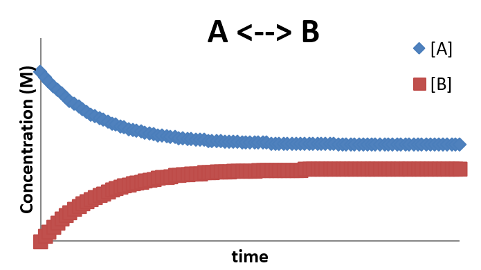
This profile is characterized by the fact that after a certain amount of time, the system achieves equilibrium and the concentrations stop changing (even though the forward and reverse reactions are still taking place. This is the nature of a dynamic equilibrium about which we speak off of the time in chemistry. The final concentrations of [A] and [B] once equilibrium is established will depend on the ratio of k1 and k-
Since the rate of formation of \(A\) (from the reverse step) is equal to the rate of consumption of \(A\) (from the forward step, the overall rate of change of the concentration of A is zero once equilibrium has been established. So it should be clear that
\[k_1[A] = k_{-1}[B] \nonumber \]
or
\[\dfrac{k_1}{k_{-1}} = \dfrac{[B]}{[A]} \nonumber \]
and the ratio o f\(k_1\) to \(k_{-1}\) gives the value of the equilibrium constant!
\(A + C \rightarrow B + C\)
Some reactions require a catalyst to mediate the conversion of reactants in to products. The definition of a catalyst is a species that must be added (it is not formed as an intermediate) shows up in the mechanism (usually in a very early step) and this ends up as part of the rate law, but is reformed later on so that it does not appear in the overall stoichiometry. If the reaction
\[A \rightarrow B \nonumber \]
is aided by a catalyst \(C\), then one possible (single-step) reaction mechanism might be
\[A + C \rightarrow B + C \nonumber \]
In this case, \(C\) is acting as a catalyst to the reaction. The rate of change of the concentrations can be found by
\[\dfrac{[A]}{dt} = -k [A][C] \nonumber \]
\[\dfrac{[B]}{dt} = k [A][C] \nonumber \]
\[\dfrac{[C]}{dt} = - k [A][C] + k [A][C] = 0 \nonumber \]
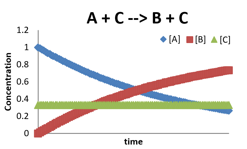
This is a very simplified picture of a catalyzed reaction. Generally a catalyzed reaction will require at least two steps:
\[A +C \rightarrow AC \nonumber \]
\[AC \rightarrow B + C \nonumber \]
Later, we will see how the steady-state approximation actually predicts the above depicted concentration profile for the two-step mechanism when \(AC\) is a short-lived species that can be treated as having a constant and small concentration.
\(A \rightarrow B \rightarrow C\)
Another important (and very common) mechanistic feature is the formation of an intermediate. This is a species that is formed in at least one of the mechanism step, but does not appear in the overall stoichiometry for the reaction. This is different from a catalyst which must be added to speed the reaction. A simple example of a reaction mechanism involving the formation of a catalyst is
\[ A \xrightarrow{k_1} B \nonumber \]
\[ B \xrightarrow{k_2} C \nonumber \]
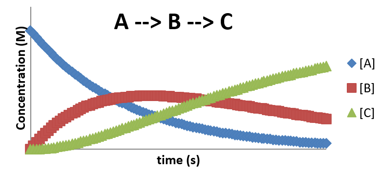
In this case, \(C\) cannot form until an appreciable concentration of the intermediate \(B\) has been created by the first step of the mechanism.
The rate of change of the concentrations of \(A\), \(B\), and \(C\) can be expressed
\[\dfrac{[A]}{dt} = -k_1 [A] \nonumber \]
\[\dfrac{[B]}{dt} = k_1 [A] - k_2 [B] \nonumber \]
\[\dfrac{[C]}{dt} = k_2 [B] \nonumber \]
The concentration profile is then shown below. Notice the delay in the formation of \(C\).
\(A \rightleftharpoons B \rightarrow C\)
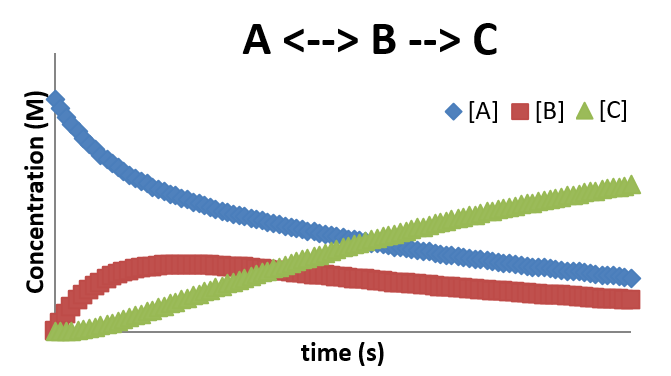
In many cases, the formation of an intermediate involves a reversible step. This step is sometimes referred to as a pre-equilibrium step since it oftentimes will establish a near equilibrium while the reaction progresses. The result of combining a pre-equilibrium with an intermediate produces a profile that shows features of both of the simpler mechanisms. An example of such a mechanism is
\[ A \xrightleftharpoons [k_1]{k_{-1}} B \nonumber \]
\[ B \xrightarrow{k_2} C \nonumber \]
In this case, the rate of change for the concentrations of \(A\), \(B\), and \(C\) can be expressed by
\[\dfrac{[A]}{dt} = -k_1 [A] + -k_{-1} [B] \nonumber \]
\[\dfrac{[B]}{dt} = k_1 [A] -k_{-1} [B] - k_2 [B] \nonumber \]
\[\dfrac{[C]}{dt} = k_2 [B] \nonumber \]
The concentration profile for this mechanism is shown below. Again, notice the delay in the production of the product \(C\), due to the requirement that the concentration of B be sufficiently high to allow the second step to occur with an appreciable rate.
\(A \rightarrow B\) and \(A \rightarrow C\)
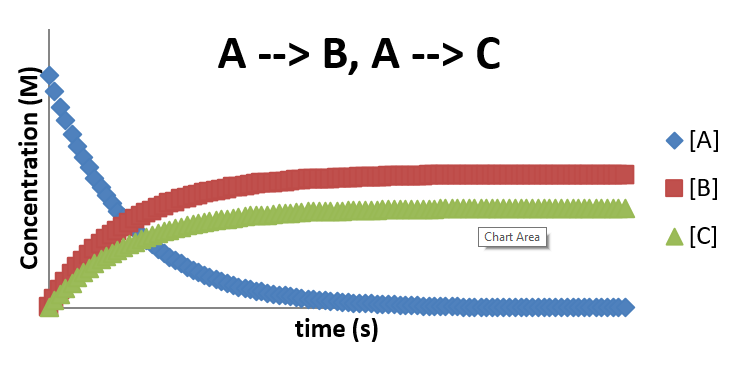
There are many cases where a reactant can follow pathways to different products (or sometimes even the same products!), and those pathways compete with one another. An example is the following simple mechanism:
\[ A \xrightarrow{k_{-1}} B \nonumber \]
\[ A \xrightarrow{k_2} C \nonumber \]
In this case, the rate of change on concentrations can be expressed as
\[\dfrac{[A]}{dt} = -k_1 [A] + -k_2 [A] \nonumber \]
\[\dfrac{[B]}{dt} = + k_1 [A] \nonumber \]
\[\dfrac{[C]}{dt} = + k_2 [A] \nonumber \]
Overall, the profile looks like two first order decompositions occurring at the same time, with the final concentration of the product formed with the larger rate constant being favored.
One of the goals of studying chemical kinetics is to understand how to alter reaction condition to favor the production of desirable reaction products. This can be accomplished by a number of means, such as alteration of concentrations, temperature, addition of catalysts, etc. Understanding the basics will (hopefully) lead to a better understanding of how concentration profiles can be altered by changing conditions.


